Add a HiGHS solver

Add a solver to generate solutions to a project prioritization problem with the HiGHS software (Huangfu and Hall 2018). This function can also be used to customize the behavior of the solver. It requires the highs package to be installed.

Usage

add_highs_solver(
  x,
  gap = 0,
  time_limit = .Machine$integer.max,
  presolve = TRUE,
  threads = 1,
  start = NULL,
  verbose = TRUE,
  control = list()
)

Arguments

x: problem() or multi_problem() object.
gap: numeric gap to optimality. This gap is relative and expresses the acceptable deviance from the optimal objective. For example, a value of 0.01 will result in the solver stopping when it has found a solution within 1% of optimality. Additionally, a value of 0 will result in the solver stopping when it has found an optimal solution. The default value is 0 (i.e., 0% from optimality).
time_limit: numeric time limit in seconds to run the optimizer. The solver will return the current best solution when this time limit is exceeded.
presolve: integer number indicating how intensively the solver should try to simplify the problem before solving it. The default value of 2 indicates to that the solver should be very aggressive in trying to simplify the problem.
threads: integer number of threads to use for the optimization algorithm. The default value of 1 will result in only one thread being used.
start: logical vector with (TRUE/FALSE) values for each action indicating if they should be selected by the starting solution. These values should be in the same order of the actions in x (i.e., per action_names(x)). Missing (NA) values can be used to indicate that the solver should automatically calculate starting values for particular actions. Defaults to NULL such that starting values are automatically determined by the solver for all actions.
verbose: logical should information be printed during optimization? Defaults to TRUE.
control: list with additional parameters for tuning the optimization process. For example, control = list(simplex_strategy = 1) could be used to set the simplex_strategy parameter. See the online documentation for information on the parameters.

Value

A problem() object with the solver added to it.

References

Huangfu Q and Hall JAJ (2018). Parallelizing the dual revised simplex method. Mathematical Programming Computation, 10: 119-142.

Examples

# load data
data(sim_projects, sim_features, sim_actions)

# build problem with highs solver
p <-
  problem(
    sim_projects, sim_actions, sim_features,
    "name", "success", "name", "cost", "name"
  ) %>%
  add_max_wtd_sum_objective(budget = 200) %>%
  add_binary_decisions() %>%
  add_highs_solver()

# print problem
print(p)
#> Project Prioritization Problem
#> actions:         F1_action, F2_action, F3_action, ... (6 actions)
#> projects:        F1_project, F2_project, F3_project, ... (6 projects)
#> features:        F1, F2, F3, ... (5 features)
#> action costs:    continuous values (between 0 and 103.226)
#> project success: proportion values (between 0.814 and 1)
#> objective:       maximum weighted sum objective
#> targets:         none specified
#> weights:         none specified
#> constraints:     none specified
#> decisions:       binary decision
#> solver:          highs solver

# solve problem
s <- solve(p)
#> MIP has 27 rows; 27 cols; 62 nonzeros; 22 integer variables (22 binary)
#> 
#> Coefficient ranges:
#> 
#>   Matrix  [9e-02, 1e+02]
#> 
#>   Cost    [1e+00, 1e+00]
#> 
#>   Bound   [5e-01, 1e+00]
#> 
#>   RHS     [1e+00, 2e+02]
#> 
#> Presolving model
#> 
#> 17 rows, 10 cols, 20 nonzeros  0s
#> 
#> 6 rows, 10 cols, 15 nonzeros  0s
#> 
#> Presolve reductions: rows 6(-21); columns 10(-17); nonzeros 15(-47) 
#> 
#> 
#> Solving MIP model with:
#>    6 rows
#>    10 cols (10 binary, 0 integer, 0 implied int., 0 continuous, 0 domain fixed)
#>    15 nonzeros
#> 
#> 
#> Src: B => Branching; C => Central rounding; F => Feasibility pump; H => Heuristic;
#> 
#>      I => Shifting; J => Feasibility jump; L => Sub-MIP; P => Empty MIP; R => Randomized rounding;
#> 
#>      S => Solve LP; T => Evaluate node; U => Unbounded; X => User solution; Y => HiGHS solution;
#> 
#>      Z => ZI Round; l => Trivial lower; p => Trivial point; u => Trivial upper; z => Trivial zero
#> 
#> 
#>         Nodes      |    B&B Tree     |            Objective Bounds              |  Dynamic Constraints |       Work      
#> Src  Proc. InQueue |  Leaves   Expl. | BestBound       BestSol              Gap |   Cuts   InLp Confl. | LpIters     Time
#> 
#> 
#>  J       0       0         0   0.00%   inf             1.680145014        Large        0      0      0         0     0.0s
#> 
#>  R       0       0         0 100.00%   2.200512004     2.190380737        0.46%        0      0      0         0     0.0s
#> 
#>          1       0         1 100.00%   2.190380737     2.190380737        0.00%        0      0      0         0     0.0s
#> 
#> 
#> Solving report
#> 
#>   Status            Optimal
#>   Primal bound      2.19038073725
#>   Dual bound        2.19038073725
#>   Gap               0%
#> 
#>   P-D integral      0.000156960239398
#> 
#>   Solution status   feasible
#> 
#>                     2.19038073725 (objective)
#>                     0 (bound viol.)
#>                     0 (int. viol.)
#>                     0 (row viol.)
#> 
#>   Timing            0.01
#> 
#>   Max sub-MIP depth 0
#>   Nodes             1
#> 
#>   Repair LPs        0
#> 
#>   LP iterations     0
#> 

# print solution
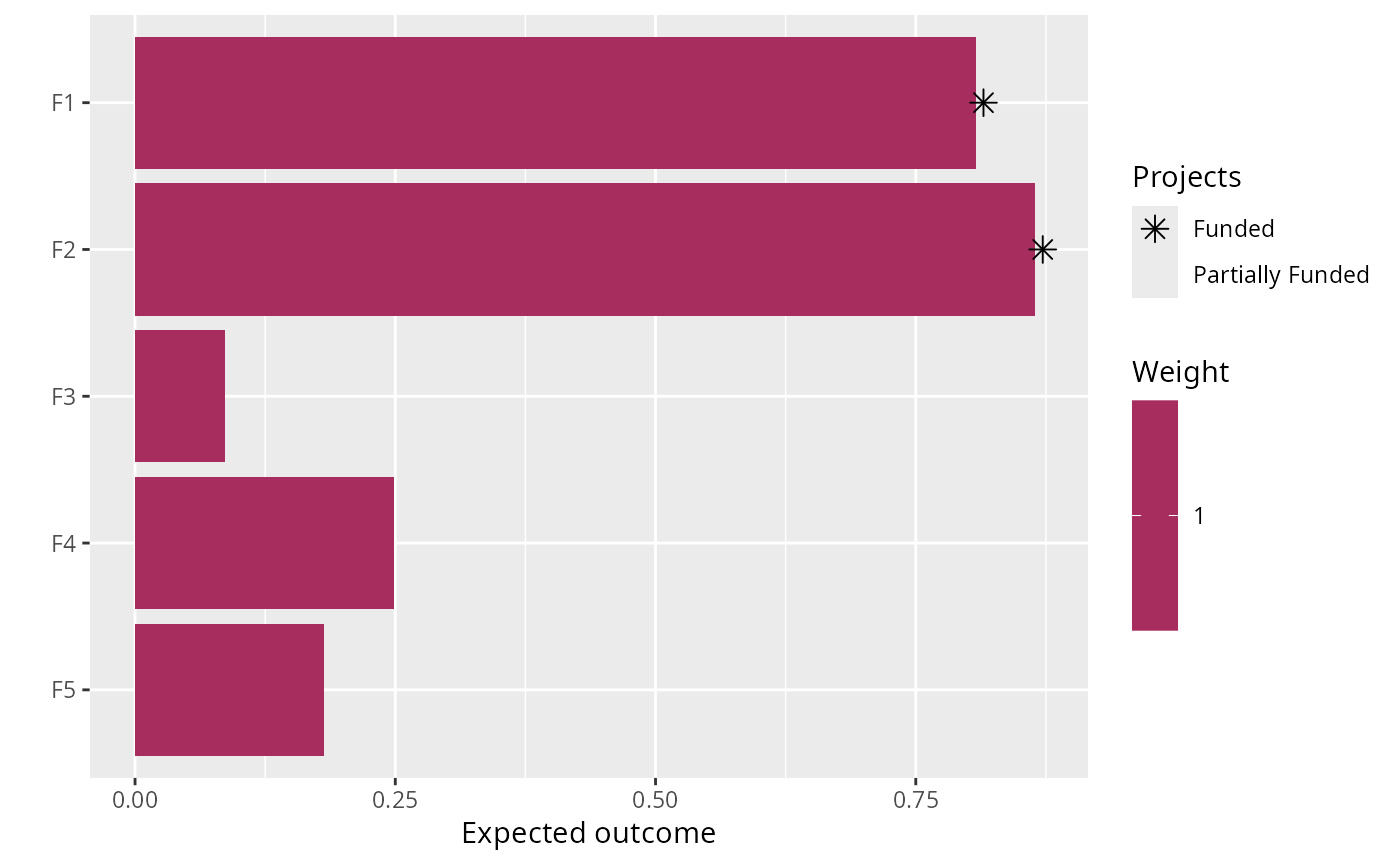
print(s)
#> # A tibble: 1 × 21
#>   solution status   cost   obj F1_action F2_action F3_action F4_action F5_action
#>      <int> <chr>   <dbl> <dbl> <lgl>     <lgl>     <lgl>     <lgl>     <lgl>    
#> 1        1 Optimal  195.  2.19 TRUE      TRUE      FALSE     FALSE     FALSE    
#> # ℹ 12 more variables: baseline_action <lgl>, F1_project <lgl>,
#> #   F2_project <lgl>, F3_project <lgl>, F4_project <lgl>, F5_project <lgl>,
#> #   baseline_project <lgl>, F1 <dbl>, F2 <dbl>, F3 <dbl>, F4 <dbl>, F5 <dbl>

# plot solution
plot(p, s)

Usage

Arguments

Value

References

See also

Examples