Add a CBC solver

Add a solver to generate solutions to a project prioritization problem with the CBC (COIN-OR branch and cut) Forrest & Lougee-Heimer 2005). This function can also be used to customize the behavior of the solver. It requires the rcbc package to be installed (only available on GitHub, see below for installation instructions).

Usage

add_cbc_solver(
  x,
  gap = 0.1,
  time_limit = .Machine$integer.max,
  presolve = 2,
  threads = 1,
  first_feasible = FALSE,
  start = NULL,
  verbose = TRUE
)

Arguments

x: problem() or multi_problem() object.
gap: numeric gap to optimality. This gap is relative and expresses the acceptable deviance from the optimal objective. For example, a value of 0.01 will result in the solver stopping when it has found a solution within 1% of optimality. Additionally, a value of 0 will result in the solver stopping when it has found an optimal solution. The default value is 0 (i.e., 0% from optimality).
time_limit: numeric time limit in seconds to run the optimizer. The solver will return the current best solution when this time limit is exceeded.
presolve: integer number indicating how intensively the solver should try to simplify the problem before solving it. Available options are: (0) disable pre-solving, (1) conservative level of pre-solving, and (2) very aggressive level of pre-solving . The default value is 2.
threads: integer number of threads to use for the optimization algorithm. The default value of 1 will result in only one thread being used.
first_feasible: logical should the first feasible solution be be returned? If first_feasible is set to TRUE, the solver will return the first solution it encounters that meets all the constraints, regardless of solution quality. Note that the first feasible solution is not an arbitrary solution, rather it is derived from the relaxed solution, and is therefore often reasonably close to optimality. Defaults to FALSE.
start: logical vector with (TRUE/FALSE) values for each action indicating if they should be selected by the starting solution. These values should be in the same order of the actions in x (i.e., per action_names(x)). Missing (NA) values can be used to indicate that the solver should automatically calculate starting values for particular actions. Defaults to NULL such that starting values are automatically determined by the solver for all actions.
verbose: logical should information be printed during optimization? Defaults to TRUE.

Value

A problem() object with the solver added to it.

Details

CBC is an open-source mixed integer programming solver that is part of the Computational Infrastructure for Operations Research (COIN-OR) project. This solver seems to have much better performance than the other open-source solvers (i.e., add_highs_solver(), add_rsymphony_solver(), add_lpsymphony_solver()) (see the Solver benchmarks vignette for details). As such, it is strongly recommended to use this solver if the Gurobi solver is not available.

Installation

The rcbc package is required to use this solver. Since the rcbc package is not available on the the Comprehensive R Archive Network (CRAN), it must be installed from its GitHub repository. To install the rcbc package, please use the following code:

if (!require(remotes)) install.packages("remotes")
remotes::install_github("dirkschumacher/rcbc")

Note that you may also need to install several dependencies – such as the Rtools software or system libraries – prior to installing the rcbc package. For further details on installing this package, please consult the online package documentation.

References

Forrest J and Lougee-Heimer R (2005) CBC User Guide. In Emerging theory, Methods, and Applications (pp. 257–277). INFORMS, Catonsville, MD. doi:10.1287/educ.1053.0020 .

Examples

# load data
data(sim_projects, sim_features, sim_actions)

# build problem with highs solver
p <-
  problem(
    sim_projects, sim_actions, sim_features,
    "name", "success", "name", "cost", "name"
  ) %>%
  add_max_wtd_sum_objective(budget = 200) %>%
  add_binary_decisions() %>%
  add_cbc_solver()

# print problem
print(p)
#> Project Prioritization Problem
#> actions:         F1_action, F2_action, F3_action, ... (6 actions)
#> projects:        F1_project, F2_project, F3_project, ... (6 projects)
#> features:        F1, F2, F3, ... (5 features)
#> action costs:    continuous values (between 0 and 103.226)
#> project success: proportion values (between 0.814 and 1)
#> objective:       maximum weighted sum objective
#> targets:         none specified
#> weights:         none specified
#> constraints:     none specified
#> decisions:       binary decision
#> solver:          cbc solver

# solve problem
s <- solve(p)

# print solution
print(s)
#> # A tibble: 1 × 21
#>   solution status   cost   obj F1_action F2_action F3_action F4_action F5_action
#>      <int> <chr>   <dbl> <dbl> <lgl>     <lgl>     <lgl>     <lgl>     <lgl>    
#> 1        1 optimal  195.  2.19 TRUE      TRUE      FALSE     FALSE     FALSE    
#> # ℹ 12 more variables: baseline_action <lgl>, F1_project <lgl>,
#> #   F2_project <lgl>, F3_project <lgl>, F4_project <lgl>, F5_project <lgl>,
#> #   baseline_project <lgl>, F1 <dbl>, F2 <dbl>, F3 <dbl>, F4 <dbl>, F5 <dbl>

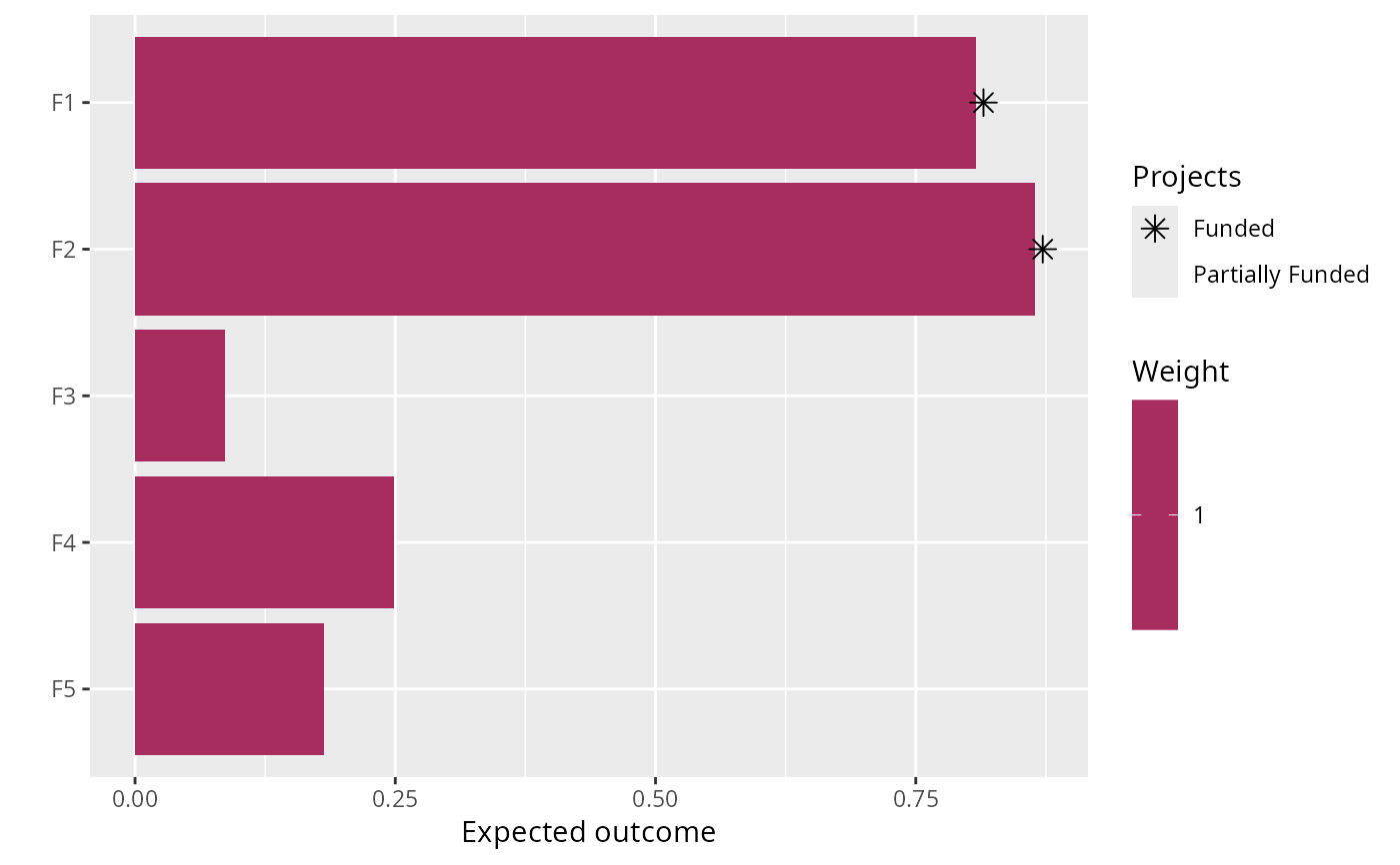
# plot solution
plot(p, s)