Add binary decisions to a project prioritization problem. This means that the optimization process aims to determine if each action should be selected for funding or not.
Arguments
- x
problem()object.
Value
A problem() object with the decisions added to it.
Details
Project prioritization problems involve making decisions about how funding will be allocated to management actions. If no decision is added to a problem then this decision type will be used by default. Currently, this is the only supported decision type.
Examples
# load data
data(sim_projects, sim_features, sim_actions)
# build problem with maximum weighted sum objective, $200 budget, and
# binary decisions
p <-
problem(
sim_projects, sim_actions, sim_features,
"name", "success", "name", "cost", "name"
) %>%
add_max_wtd_sum_objective(budget = 200) %>%
add_binary_decisions()
# print problem
print(p)
#> Project Prioritization Problem
#> actions: F1_action, F2_action, F3_action, ... (6 actions)
#> projects: F1_project, F2_project, F3_project, ... (6 projects)
#> features: F1, F2, F3, ... (5 features)
#> action costs: continuous values (between 0 and 103.226)
#> project success: proportion values (between 0.814 and 1)
#> objective: maximum weighted sum objective
#> targets: none specified
#> weights: none specified
#> constraints: none specified
#> decisions: binary decision
#> solver: none specified
# solve problem
s <- solve(p)
#> Set parameter Username
#> Set parameter LicenseID to value 2806834
#> Set parameter TimeLimit to value 2147483647
#> Set parameter MIPGap to value 0
#> Set parameter ScaleFlag to value 2
#> Set parameter NumericFocus to value 1
#> Set parameter Presolve to value 2
#> Set parameter Threads to value 1
#> Set parameter PoolSolutions to value 1
#> Set parameter PoolSearchMode to value 2
#> Academic license - for non-commercial use only - expires 2027-04-14
#> Gurobi Optimizer version 13.0.1 build v13.0.1rc0 (linux64 - "Ubuntu 24.04.2 LTS")
#>
#> CPU model: 11th Gen Intel(R) Core(TM) i7-1185G7 @ 3.00GHz, instruction set [SSE2|AVX|AVX2|AVX512]
#> Thread count: 4 physical cores, 8 logical processors, using up to 1 threads
#>
#> Non-default parameters:
#> TimeLimit 2147483647
#> MIPGap 0
#> ScaleFlag 2
#> NumericFocus 1
#> Presolve 2
#> Threads 1
#> PoolSolutions 1
#> PoolSearchMode 2
#>
#> Optimize a model with 27 rows, 27 columns and 62 nonzeros (Max)
#> Model fingerprint: 0x3c076626
#> Model has 5 linear objective coefficients
#> Variable types: 5 continuous, 22 integer (22 binary)
#> Coefficient statistics:
#> Matrix range [9e-02, 1e+02]
#> Objective range [1e+00, 1e+00]
#> Bounds range [5e-01, 1e+00]
#> RHS range [1e+00, 2e+02]
#>
#> Found heuristic solution: objective 1.4456093
#> Presolve removed 16 rows and 12 columns
#> Presolve time: 0.00s
#> Presolved: 11 rows, 15 columns, 25 nonzeros
#> Variable types: 0 continuous, 15 integer (15 binary)
#> Root relaxation presolved: 11 rows, 15 columns, 25 nonzeros
#>
#>
#> Root relaxation: objective 2.190381e+00, 12 iterations, 0.00 seconds (0.00 work units)
#>
#> Nodes | Current Node | Objective Bounds | Work
#> Expl Unexpl | Obj Depth IntInf | Incumbent BestBd Gap | It/Node Time
#>
#> * 0 0 0 2.1903807 2.19038 0.00% - 0s
#>
#> Explored 1 nodes (12 simplex iterations) in 0.00 seconds (0.00 work units)
#> Thread count was 1 (of 8 available processors)
#>
#> Solution count 1: 2.19038
#> No other solutions better than 2.19038
#>
#> Optimal solution found (tolerance 0.00e+00)
#> Best objective 2.190380737245e+00, best bound 2.190380737245e+00, gap 0.0000%
# print solution
print(s)
#> # A tibble: 1 × 21
#> solution status cost obj F1_action F2_action F3_action F4_action F5_action
#> <int> <chr> <dbl> <dbl> <lgl> <lgl> <lgl> <lgl> <lgl>
#> 1 1 OPTIMAL 195. 2.19 TRUE TRUE FALSE FALSE FALSE
#> # ℹ 12 more variables: baseline_action <lgl>, F1_project <lgl>,
#> # F2_project <lgl>, F3_project <lgl>, F4_project <lgl>, F5_project <lgl>,
#> # baseline_project <lgl>, F1 <dbl>, F2 <dbl>, F3 <dbl>, F4 <dbl>, F5 <dbl>
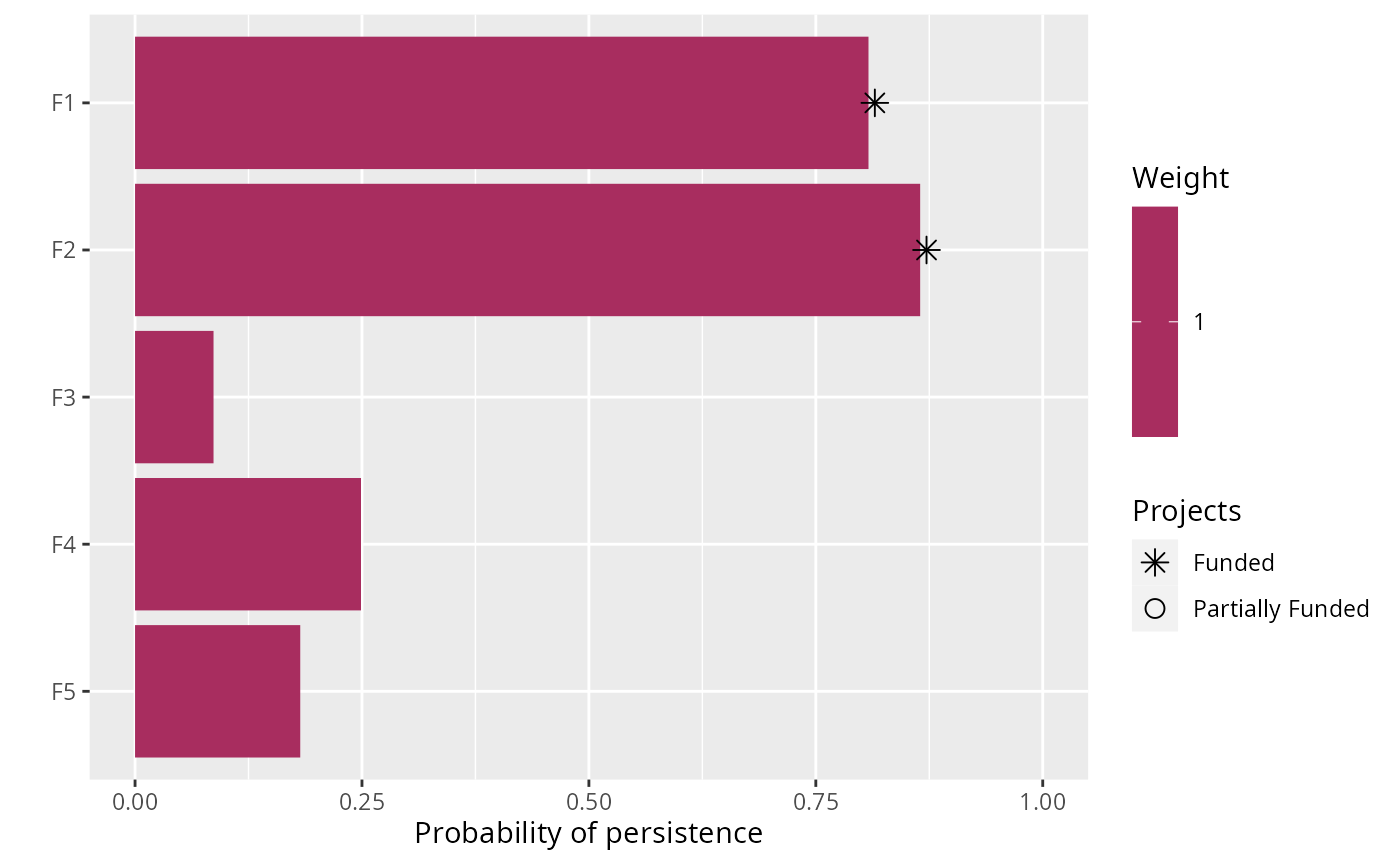
# plot solution
plot(p, s)