Project prioritization problem

Create a project prioritization problem. This function is used to specify the underlying data used in a prioritization problem: the projects, the management actions, and the features that need to be conserved (e.g., species, ecosystems). After constructing this ProjectProblem-class object, it can be customized using objectives, targets, weights, constraints, decisions and solvers. After building the problem, the solve() function can be used to identify solutions.

Usage

problem(
  projects,
  actions,
  features,
  project_name_column,
  project_success_column,
  action_name_column,
  action_cost_column,
  feature_name_column,
  adjust_for_baseline = TRUE,
  baseline_project_name = NULL
)

Arguments

projects

base::data.frame() or tibble::tibble() table containing project data. Here, each row should correspond to a different project and columns should contain data that correspond to each project. It should contain data that denote (i) the name of each project (specified in the argument to project_name_column), (ii) the probability that each project will succeed if all of its actions are funded (specified in the argument to project_success_column), (iii) the outcome (e.g., probability of species' persistence, amount of land covered by an ecosystem) that would be expected for each feature assuming that the project if successfully completed (using a column for each feature), and (iv) and which actions are associated with which projects (using a column for each action). Additionally, projects must have a baseline project (with a zero cost value) that represents the outcome that would be expected if no other project is successfully completed for each feature. Since each feature is assigned the greatest outcome value based on the projects selected for funding in a solution, the combined benefits of multiple projects can be specified by creating additional projects that represent "combined projects". For instance, a habitat restoration project might cost $100 and mean that a feature has a 40% chance of persisting, and a pest eradication project might cost $50 and mean that a feature has a 60% chance of persisting. Due to non-linear effects, funding both of these projects might mean that a species has a 90% chance of persistence. This can be accounted for by creating a third project, representing the funding of both projects, which costs $150 and provides a 90% chance of persistence.

actions

base::data.frame() or tibble::tibble() table containing the action data. Here, each row should correspond to a different action and columns should contain data that correspond to each action. At a minimum, this object should contain data that denote (i) the name of each action (specified in the argument to action_name_column), (ii) the cost of each action (specified in the argument to action_cost_column). Optionally, it may also contain data that indicate actions should be (iii) locked in or (iv) locked out (see add_locked_in_action_constraints() and add_locked_out_action_constraints()). It should also contain a zero-cost baseline action that is associated with the baseline project.

features

base::data.frame() or tibble::tibble() table containing the feature data. Here, each row should correspond to a different feature and columns should contain data that correspond to each feature. At a minimum, this object should contain data that denote (i) the name of each feature (specified in the argument to feature_name_column). Optionally, it may also contain (ii) the weight for each feature or (iii) persistence targets for each feature.

project_name_column

character name of column that contains the name for each conservation project. This argument corresponds to the projects table. Note that the project names must not contain any duplicates or missing values.

project_success_column

character name of column that indicates the probability that each project will succeed. This argument corresponds to the argument to projects table. This column must have numeric values which range between zero and one. No missing values are permitted.

action_name_column

character name of column that contains the name for each management action. This argument corresponds to the actions table. Note that the project names must not contain any duplicates or missing values.

action_cost_column

character name of column that indicates the cost for funding each action. This argument corresponds to the argument to actions table. This column must have numeric values which are equal to or greater than zero. No missing values are permitted.

feature_name_column

character name of the column that contains the name for each feature. This argument corresponds to the feature table. Note that the feature names must not contain any duplicates or missing values.

adjust_for_baseline

logical should the expected outcome associated with a particular project be adjusted to account for the outcome associated with the baseline project in the event that the particular project is not successfully competed? This should almost always be set to TRUE to ensure that the calculations do not assume that failing to successfully complete a funded project will result in an outcome with a value of zero (which is often worse than the baseline project). Defaults to TRUE.

baseline_project_name

character name of the baseline project. Defaults to NULL such that the baseline project name is automatically inferred based on which action has a zero cost. Note that if multiple actions have zero costs, then baseline_project_name must be specified.

Value

A new ProjectProblem object.

Details

A project prioritization problem has actions, projects, and features. Features are the biological entities that need to be conserved (e.g., species, populations, ecosystems). Actions are real-world management actions that can be implemented to enhance biodiversity (e.g., habitat restoration, monitoring, pest eradication). Each action should have a known cost, and this usually means that each action should have a defined spatial extent and time period (though this is not necessary). Conservation projects are groups of management actions (they can also comprise a singular action too), and each project is associated with a probability of success if all of its associated actions are funded. To determine which projects should be funded, each project is associated with an probability of persistence for the features that they benefit. These values should indicate the probability that each feature will persist if only that project funded and not the additional benefit relative to the baseline project. Missing (NA) values should be used to indicate which projects do not enhance the probability of certain features.

The goal of a project prioritization exercise is then to identify which management actions—and as a consequence which conservation projects—should be funded. Broadly speaking, the goal of an optimization problem is to minimize (or maximize) an objective unction given a set of control variables and decision variables that are subject to a series of constraints. In the context of project prioritization problems, the objective is usually some measure of utility (e.g., the net probability of each feature persisting into the future), the control variables determine which actions should be funded or not, the decision variables contain additional information needed to ensure correct calculations, and the constraints impose limits such as the total budget available for funding management actions. For more information on the mathematical formulations used in this package, please refer to the manual entries for the available objectives (listed in objectives).

See also

constraints, decisions, objectives, solvers, targets, weights, solution_statistics(), plot.ProjectProblem().

Examples

# load data
data(sim_projects, sim_features, sim_actions)

# print project data
print(sim_projects)
#> # A tibble: 6 × 13
#>   name           success     F1     F2      F3     F4     F5 F1_action F2_action
#>   <chr>            <dbl>  <dbl>  <dbl>   <dbl>  <dbl>  <dbl> <lgl>     <lgl>    
#> 1 F1_project       0.919  0.791 NA     NA      NA     NA     TRUE      FALSE    
#> 2 F2_project       0.923 NA      0.888 NA      NA     NA     FALSE     TRUE     
#> 3 F3_project       0.829 NA     NA      0.502  NA     NA     FALSE     FALSE    
#> 4 F4_project       0.848 NA     NA     NA       0.690 NA     FALSE     FALSE    
#> 5 F5_project       0.814 NA     NA     NA      NA      0.617 FALSE     FALSE    
#> 6 baseline_proj…   1      0.298  0.250  0.0865  0.249  0.182 FALSE     FALSE    
#> # ℹ 4 more variables: F3_action <lgl>, F4_action <lgl>, F5_action <lgl>,
#> #   baseline_action <lgl>

# print action data
print(sim_features)
#> # A tibble: 5 × 2
#>   name  weight
#>   <chr>  <dbl>
#> 1 F1     0.211
#> 2 F2     0.211
#> 3 F3     0.221
#> 4 F4     0.630
#> 5 F5     1.59 

# print feature data
print(sim_actions)
#> # A tibble: 6 × 4
#>   name             cost locked_in locked_out
#>   <chr>           <dbl> <lgl>     <lgl>     
#> 1 F1_action        94.4 FALSE     FALSE     
#> 2 F2_action       101.  FALSE     FALSE     
#> 3 F3_action       103.  TRUE      FALSE     
#> 4 F4_action        99.2 FALSE     FALSE     
#> 5 F5_action        99.9 FALSE     TRUE      
#> 6 baseline_action   0   FALSE     FALSE     

# build problem
p <-
  problem(
    sim_projects, sim_actions, sim_features,
    "name", "success", "name", "cost", "name"
  ) %>%
  add_max_wtd_sum_objective(budget = 400) %>%
  add_feature_weights("weight") %>%
  add_binary_decisions()

# print problem
print(p)
#> Project Prioritization Problem
#> actions:         F1_action, F2_action, F3_action, ... (6 actions)
#> projects:        F1_project, F2_project, F3_project, ... (6 projects)
#> features:        F1, F2, F3, ... (5 features)
#> action costs:    continuous values (between 0 and 103.226)
#> project success: proportion values (between 0.814 and 1)
#> objective:       maximum weighted sum objective
#> targets:         none specified
#> weights:         feature weights
#> constraints:     none specified
#> decisions:       binary decision
#> solver:          none specified

# solve problem
s <- solve(p)
#> Set parameter Username
#> Set parameter LicenseID to value 2806834
#> Set parameter TimeLimit to value 2147483647
#> Set parameter MIPGap to value 0
#> Set parameter ScaleFlag to value 2
#> Set parameter NumericFocus to value 1
#> Set parameter Presolve to value 2
#> Set parameter Threads to value 1
#> Set parameter PoolSolutions to value 1
#> Set parameter PoolSearchMode to value 2
#> Academic license - for non-commercial use only - expires 2027-04-14
#> Gurobi Optimizer version 13.0.1 build v13.0.1rc0 (linux64 - "Ubuntu 24.04.2 LTS")
#> 
#> CPU model: 11th Gen Intel(R) Core(TM) i7-1185G7 @ 3.00GHz, instruction set [SSE2|AVX|AVX2|AVX512]
#> Thread count: 4 physical cores, 8 logical processors, using up to 1 threads
#> 
#> Non-default parameters:
#> TimeLimit  2147483647
#> MIPGap  0
#> ScaleFlag  2
#> NumericFocus  1
#> Presolve  2
#> Threads  1
#> PoolSolutions  1
#> PoolSearchMode  2
#> 
#> Optimize a model with 27 rows, 27 columns and 62 nonzeros (Max)
#> Model fingerprint: 0x85f2486a
#> Model has 5 linear objective coefficients
#> Variable types: 5 continuous, 22 integer (22 binary)
#> Coefficient statistics:
#>   Matrix range     [9e-02, 1e+02]
#>   Objective range  [2e-01, 2e+00]
#>   Bounds range     [5e-01, 1e+00]
#>   RHS range        [1e+00, 4e+02]
#> 
#> Found heuristic solution: objective 0.6654645
#> Presolve removed 16 rows and 12 columns
#> Presolve time: 0.00s
#> Presolved: 11 rows, 15 columns, 24 nonzeros
#> Variable types: 0 continuous, 15 integer (15 binary)
#> Root relaxation presolved: 11 rows, 15 columns, 24 nonzeros
#> 
#> 
#> Root relaxation: objective 1.749045e+00, 11 iterations, 0.00 seconds (0.00 work units)
#> 
#>     Nodes    |    Current Node    |     Objective Bounds      |     Work
#>  Expl Unexpl |  Obj  Depth IntInf | Incumbent    BestBd   Gap | It/Node Time
#> 
#> *    0     0               0       1.7490448    1.74904  0.00%     -    0s
#> 
#> Explored 1 nodes (11 simplex iterations) in 0.00 seconds (0.00 work units)
#> Thread count was 1 (of 8 available processors)
#> 
#> Solution count 1: 1.74904 
#> No other solutions better than 1.74904
#> 
#> Optimal solution found (tolerance 0.00e+00)
#> Best objective 1.749044775334e+00, best bound 1.749044775334e+00, gap 0.0000%

# print output
print(s)
#> # A tibble: 1 × 21
#>   solution status   cost   obj F1_action F2_action F3_action F4_action F5_action
#>      <int> <chr>   <dbl> <dbl> <lgl>     <lgl>     <lgl>     <lgl>     <lgl>    
#> 1        1 OPTIMAL  395.  1.75 TRUE      TRUE      FALSE     TRUE      TRUE     
#> # ℹ 12 more variables: baseline_action <lgl>, F1_project <lgl>,
#> #   F2_project <lgl>, F3_project <lgl>, F4_project <lgl>, F5_project <lgl>,
#> #   baseline_project <lgl>, F1 <dbl>, F2 <dbl>, F3 <dbl>, F4 <dbl>, F5 <dbl>

# print which actions are funded in the solution
s[, sim_actions$name, drop = FALSE]
#> # A tibble: 1 × 6
#>   F1_action F2_action F3_action F4_action F5_action baseline_action
#>   <lgl>     <lgl>     <lgl>     <lgl>     <lgl>     <lgl>          
#> 1 TRUE      TRUE      FALSE     TRUE      TRUE      TRUE           

# print the expected probability of persistence for each feature
# if the solution were implemented
s[, sim_features$name, drop = FALSE]
#> # A tibble: 1 × 5
#>      F1    F2     F3    F4    F5
#>   <dbl> <dbl>  <dbl> <dbl> <dbl>
#> 1 0.808 0.865 0.0865 0.688 0.592

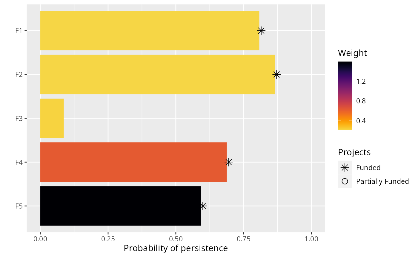
# visualize solution
plot(p, s)