Add a solver to generate solutions to a project prioritization problem based on random selection. Although prioritizations should be developed using optimization routines, a portfolio of randomly generated solutions can be useful for evaluating the effectiveness of an optimized solution.
Arguments
- x
problem()ormulti_problem()object.- number_solutions
integernumber of solutions desired. Defaults to 1. Note that the number of returned solutions can sometimes be less than the argument tonumber_solutionsdepending on the argument tosolution_pool_method, for example if 100 solutions are requested but only 10 unique solutions exist, then only 10 solutions will be returned.- verbose
logicalshould information be printed during optimization? Defaults toTRUE.
Value
A problem() object with the solver added to it.
Details
The algorithm used to randomly generate solutions depends on the the objective specified for the project prioritization problem.
The following steps are used for objectives that maximize benefit subject to
budgetary constraints (e.g., add_max_wtd_sum_objective()).
All locked in and zero-cost actions are initially selected for funding (excepting actions which are locked out).
A project—and all of its associated actions—is randomly selected for funding (excepting projects associated with locked out actions, and projects which would cause the budget to be exceeded when added to the existing set of selected actions).
The previous step is repeated until no more projects can be selected for funding without the total cost of the prioritized actions exceeding the budget.
The following steps are used for objectives that minimize cost subject to
biodiversity constraints (i.e., add_min_set_objective().
All locked in and zero-cost actions are initially selected for funding (excepting actions which are locked out).
A project—and all of its associated actions—is randomly selected for funding (excepting projects associated with locked out actions, and projects which would cause the budget to be exceeded when added to the existing set of selected actions).
The previous step is repeated until all of the persistence targets are met.
Examples
# load data
data(sim_projects, sim_features, sim_actions)
# build problem with random solver, and generate 100 random solutions
p1 <-
problem(
sim_projects, sim_actions, sim_features,
"name", "success", "name", "cost", "name"
) %>%
add_max_wtd_sum_objective(budget = 200) %>%
add_binary_decisions() %>%
add_random_solver(number_solutions = 100)
# print problem
print(p1)
#> Project Prioritization Problem
#> actions: F1_action, F2_action, F3_action, ... (6 actions)
#> projects: F1_project, F2_project, F3_project, ... (6 projects)
#> features: F1, F2, F3, ... (5 features)
#> action costs: continuous values (between 0 and 103.226)
#> project success: proportion values (between 0.814 and 1)
#> objective: maximum weighted sum objective
#> targets: none specified
#> weights: none specified
#> constraints: none specified
#> decisions: binary decision
#> solver: random solver
# solve problem
s1 <- solve(p1)
# print solutions
print(s1)
#> # A tibble: 100 × 21
#> solution status cost obj F1_action F2_action F3_action F4_action F5_action
#> <int> <chr> <dbl> <dbl> <lgl> <lgl> <lgl> <lgl> <lgl>
#> 1 1 NA 194. 1.99 TRUE FALSE FALSE FALSE TRUE
#> 2 2 NA 194. 2.01 TRUE FALSE FALSE TRUE FALSE
#> 3 3 NA 198. 1.96 TRUE FALSE TRUE FALSE FALSE
#> 4 4 NA 198. 1.96 TRUE FALSE TRUE FALSE FALSE
#> 5 5 NA 199. 1.91 FALSE FALSE FALSE TRUE TRUE
#> 6 6 NA 194. 1.99 TRUE FALSE FALSE FALSE TRUE
#> 7 7 NA 198. 1.96 TRUE FALSE TRUE FALSE FALSE
#> 8 8 NA 198. 1.96 TRUE FALSE TRUE FALSE FALSE
#> 9 9 NA 198. 1.96 TRUE FALSE TRUE FALSE FALSE
#> 10 10 NA 195. 2.19 TRUE TRUE FALSE FALSE FALSE
#> # ℹ 90 more rows
#> # ℹ 12 more variables: baseline_action <lgl>, F1_project <lgl>,
#> # F2_project <lgl>, F3_project <lgl>, F4_project <lgl>, F5_project <lgl>,
#> # baseline_project <lgl>, F1 <dbl>, F2 <dbl>, F3 <dbl>, F4 <dbl>, F5 <dbl>
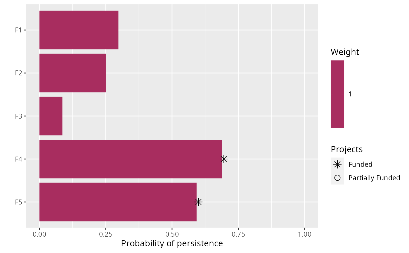
# plot first random solution
plot(p1, s1)
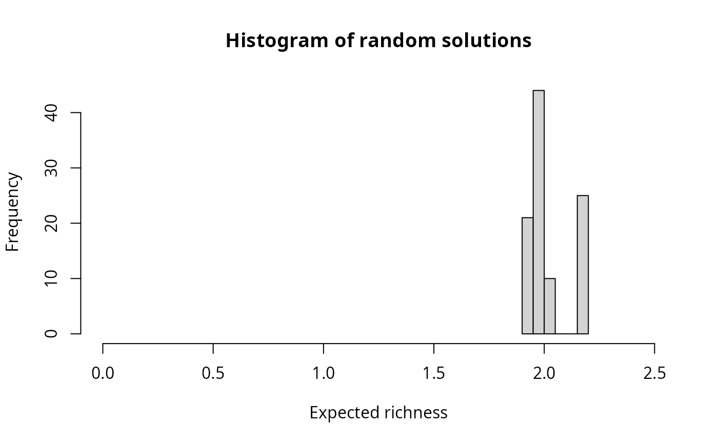
 # plot histogram of the objective values for the random solutions
# according to the weighted sum objective
hist(
s1$obj,
xlab = "Expected outcome", xlim = c(0, 2.5),
main = "Histogram of random solutions"
)
# plot histogram of the objective values for the random solutions
# according to the weighted sum objective
hist(
s1$obj,
xlab = "Expected outcome", xlim = c(0, 2.5),
main = "Histogram of random solutions"
)
 # since the objective values don't tell us much about the quality of the
# solutions, we can find the optimal solution and calculate how different
# each of the random solutions is from optimality
# find the optimal objective value using an exact algorithms solver
s2 <- p1 %>%
add_default_solver() %>%
solve()
#> Warning: Overwriting previously defined solver.
#> Set parameter Username
#> Set parameter LicenseID to value 2806834
#> Set parameter TimeLimit to value 2147483647
#> Set parameter MIPGap to value 0
#> Set parameter ScaleFlag to value 2
#> Set parameter NumericFocus to value 1
#> Set parameter Presolve to value 2
#> Set parameter Threads to value 1
#> Set parameter PoolSolutions to value 1
#> Set parameter PoolSearchMode to value 2
#> Academic license - for non-commercial use only - expires 2027-04-14
#> Gurobi Optimizer version 13.0.1 build v13.0.1rc0 (linux64 - "Ubuntu 24.04.2 LTS")
#>
#> CPU model: 11th Gen Intel(R) Core(TM) i7-1185G7 @ 3.00GHz, instruction set [SSE2|AVX|AVX2|AVX512]
#> Thread count: 4 physical cores, 8 logical processors, using up to 1 threads
#>
#> Non-default parameters:
#> TimeLimit 2147483647
#> MIPGap 0
#> ScaleFlag 2
#> NumericFocus 1
#> Presolve 2
#> Threads 1
#> PoolSolutions 1
#> PoolSearchMode 2
#>
#> Optimize a model with 27 rows, 27 columns and 62 nonzeros (Max)
#> Model fingerprint: 0x3c076626
#> Model has 5 linear objective coefficients
#> Variable types: 5 continuous, 22 integer (22 binary)
#> Coefficient statistics:
#> Matrix range [9e-02, 1e+02]
#> Objective range [1e+00, 1e+00]
#> Bounds range [5e-01, 1e+00]
#> RHS range [1e+00, 2e+02]
#>
#> Found heuristic solution: objective 1.4456093
#> Presolve removed 16 rows and 12 columns
#> Presolve time: 0.00s
#> Presolved: 11 rows, 15 columns, 25 nonzeros
#> Variable types: 0 continuous, 15 integer (15 binary)
#> Root relaxation presolved: 11 rows, 15 columns, 25 nonzeros
#>
#>
#> Root relaxation: objective 2.190381e+00, 12 iterations, 0.00 seconds (0.00 work units)
#>
#> Nodes | Current Node | Objective Bounds | Work
#> Expl Unexpl | Obj Depth IntInf | Incumbent BestBd Gap | It/Node Time
#>
#> * 0 0 0 2.1903807 2.19038 0.00% - 0s
#>
#> Explored 1 nodes (12 simplex iterations) in 0.00 seconds (0.00 work units)
#> Thread count was 1 (of 8 available processors)
#>
#> Solution count 1: 2.19038
#> No other solutions better than 2.19038
#>
#> Optimal solution found (tolerance 0.00e+00)
#> Best objective 2.190380737245e+00, best bound 2.190380737245e+00, gap 0.0000%
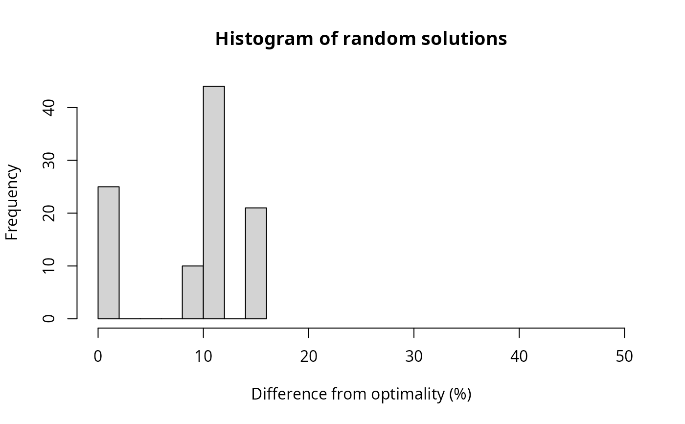
# create new column in s1 with percent difference from optimality
s1$optimality_diff <- ((s2$obj - s1$obj) / s1$obj) * 100
# plot histogram showing the quality of the random solutions
# higher numbers indicate worse solutions
hist(
s1$optimality_diff,
xlab = "Difference from optimality (%)",
main = "Histogram of random solutions", xlim = c(0, 50)
)
# since the objective values don't tell us much about the quality of the
# solutions, we can find the optimal solution and calculate how different
# each of the random solutions is from optimality
# find the optimal objective value using an exact algorithms solver
s2 <- p1 %>%
add_default_solver() %>%
solve()
#> Warning: Overwriting previously defined solver.
#> Set parameter Username
#> Set parameter LicenseID to value 2806834
#> Set parameter TimeLimit to value 2147483647
#> Set parameter MIPGap to value 0
#> Set parameter ScaleFlag to value 2
#> Set parameter NumericFocus to value 1
#> Set parameter Presolve to value 2
#> Set parameter Threads to value 1
#> Set parameter PoolSolutions to value 1
#> Set parameter PoolSearchMode to value 2
#> Academic license - for non-commercial use only - expires 2027-04-14
#> Gurobi Optimizer version 13.0.1 build v13.0.1rc0 (linux64 - "Ubuntu 24.04.2 LTS")
#>
#> CPU model: 11th Gen Intel(R) Core(TM) i7-1185G7 @ 3.00GHz, instruction set [SSE2|AVX|AVX2|AVX512]
#> Thread count: 4 physical cores, 8 logical processors, using up to 1 threads
#>
#> Non-default parameters:
#> TimeLimit 2147483647
#> MIPGap 0
#> ScaleFlag 2
#> NumericFocus 1
#> Presolve 2
#> Threads 1
#> PoolSolutions 1
#> PoolSearchMode 2
#>
#> Optimize a model with 27 rows, 27 columns and 62 nonzeros (Max)
#> Model fingerprint: 0x3c076626
#> Model has 5 linear objective coefficients
#> Variable types: 5 continuous, 22 integer (22 binary)
#> Coefficient statistics:
#> Matrix range [9e-02, 1e+02]
#> Objective range [1e+00, 1e+00]
#> Bounds range [5e-01, 1e+00]
#> RHS range [1e+00, 2e+02]
#>
#> Found heuristic solution: objective 1.4456093
#> Presolve removed 16 rows and 12 columns
#> Presolve time: 0.00s
#> Presolved: 11 rows, 15 columns, 25 nonzeros
#> Variable types: 0 continuous, 15 integer (15 binary)
#> Root relaxation presolved: 11 rows, 15 columns, 25 nonzeros
#>
#>
#> Root relaxation: objective 2.190381e+00, 12 iterations, 0.00 seconds (0.00 work units)
#>
#> Nodes | Current Node | Objective Bounds | Work
#> Expl Unexpl | Obj Depth IntInf | Incumbent BestBd Gap | It/Node Time
#>
#> * 0 0 0 2.1903807 2.19038 0.00% - 0s
#>
#> Explored 1 nodes (12 simplex iterations) in 0.00 seconds (0.00 work units)
#> Thread count was 1 (of 8 available processors)
#>
#> Solution count 1: 2.19038
#> No other solutions better than 2.19038
#>
#> Optimal solution found (tolerance 0.00e+00)
#> Best objective 2.190380737245e+00, best bound 2.190380737245e+00, gap 0.0000%
# create new column in s1 with percent difference from optimality
s1$optimality_diff <- ((s2$obj - s1$obj) / s1$obj) * 100
# plot histogram showing the quality of the random solutions
# higher numbers indicate worse solutions
hist(
s1$optimality_diff,
xlab = "Difference from optimality (%)",
main = "Histogram of random solutions", xlim = c(0, 50)
)