Add maximum weighted sum objective
Source:R/add_max_wtd_sum_objective.R
add_max_wtd_sum_objective.RdAdd an objective to a project prioritization problem based on
maximizing the weighted sum of expected outcomes associated with the
features, whilst ensuring that the cost of the
solution is within a pre-specified budget
(Joseph, Maloney & Possingham 2009).
Weights can be used to specify the relative importance of conserving specific
features (see add_feature_weights()).
Although this objective is conceptually
similar to maximizing species richness (add_max_richness_objective()
it is designed to work for features that are not associated with
probabilistic outcomes.
Arguments
- x
problem()object.- budget
numericvalue representing the maximum amount of total expenditure for funding actions.
Value
A problem() with the objective added to it.
Details
A problem objective is used to specify the overall goal of the project prioritization problem. Here, this objective seeks to find the set of actions that maximizes the weighted sum of the expected outcomes (e.g., probability of persistence, population size, amount of habitat) associated with the features (e.g., populations, species, ecosystems) within a pre-specified budget. Let \(I\) represent the set of conservation actions (indexed by \(i\)). Let \(C_i\) denote the cost for funding action \(i\), and let \(m\) denote the maximum expenditure (i.e., the budget). Also, let \(F\) represent each feature (indexed by \(f\)), \(W_f\) represent the weight for each feature \(f\) (defaults to one for each feature unless specified otherwise), and \(E_f\) denote the expected outcome for each feature given the funded conservation projects.
To guide the prioritization, the conservation actions are organized into
conservation projects. Let \(J\) denote the set of conservation projects
(indexed by \(j\)), and let \(A_{ij}\) denote which actions
\(i \in I\) comprise each conservation project
\(j \in J\) using zeros and ones. Next, let \(P_j\) represent
the probability of project \(j\) being successful if it is funded. Also,
let \(B_{fj}\) denote the outcome for each feature
\(f \in F\) associated with the project \(j \in J\)
assuming that all of the actions comprising project \(j\) are funded
and that project is allocated to feature \(f\). For convenience,
let \(Q_{fj}\) denote the expected outcome for each
\(f \in F\) associated with the project \(j \in J\)
if the project is funded. If the argument
to adjust_for_baseline in the problem function was set to
TRUE, and this is the default behavior, then
\(Q_{fj} = (P_{j} \times B_{fj}) + \bigg(\big(1 - (P_{j} B_{fj})\big)
\times (P_{n} \times B_{fn})\bigg)\), where n corresponds to the
baseline "do nothing" project. This means that the expected outcome
for a feature given that a project is funded and allocated to the feature
depends on (i) the probability of the project succeeding, (ii) the
outcome for the feature if the project succeeds,
and (iii) the outcome for the feature if the project fails
(per the baseline project).
Otherwise, if the argument is set to FALSE, then
\(Q_{fj} = P_{j} \times B_{fj}\).
The binary control variables \(X_i\) in this problem indicate whether each project \(i \in I\) is funded or not. The decision variables in this problem are the \(Y_{j}\), \(Z_{fj}\), and \(E_f\) variables. Specifically, the binary \(Y_{j}\) variables indicate if project \(j\) is funded or not based on which actions are funded; and the binary \(Z_{fj}\) variables indicate if project \(j\) is used to manage feature \(f\) or not.
Now that we have defined all the data and variables, we can formulate the problem. For convenience, let the symbol used to denote each set also represent its cardinality (e.g., if there are ten features, let \(F\) represent the set of ten features and also the number ten).
$$ \mathrm{Maximize} \space \sum_{f = 0}^{F} E_f W_f \space \mathrm{(eqn \space 1a)} \\ \mathrm{Subject \space to} \sum_{i = 0}^{I} C_i \leq m \space \mathrm{(eqn \space 1b)} \\ E_f = \sum_{j = 0}^{J} Z_{fj} Q_{fj} \space \forall \space f \in F \space \mathrm{(eqn \space 1c)} \\ Z_{fj} \leq Y_{j} \space \forall \space j \in J \space \mathrm{(eqn \space 1d)} \\ \sum_{j = 0}^{J} Z_{fj} \times \mathrm{ceil}(Q_{fj}) = 1 \space \forall \space f \in F \space \mathrm{(eqn \space 1e)} \\ A_{ij} Y_{j} \leq X_{i} \space \forall \space i \in I, j \in J \space \mathrm{(eqn \space 1f)} \\ E_{f} \geq 0 \space \forall \space f \in F \space \mathrm{(eqn \space 1g)} \\ X_{i}, Y_{j}, Z_{fj} \in \{0, 1\} \space \forall \space i \in I, j \in J, f \in F \space \mathrm{(eqn \space 1h)} $$
The objective (eqn 1a) is to maximize the weighted sum of the expected outcome values for the features. Constraint (eqn 1b) limits the maximum expenditure (i.e., ensures that the cost of the funded actions do not exceed the budget). Constraints (eqn 1c) calculate the expected outcome for each feature according to their allocated project. Constraints (eqn 1d) ensure that feature can only be allocated to projects that have all of their actions funded. Constraints (eqn 1e) state that each feature can only be allocated to a single project. Constraints (eqn 1f) ensure that a project cannot be funded unless all of its actions are funded. Constraints (eqns 1g) ensure that the expected outcome variables (\(E_f\)) are greater than zero. Constraints (eqns 1h) ensure that the action funding (\(X_i\)), project funding (\(Y_j\)), and project allocation (\(Z_{fj}\)) variables are binary.
References
Joseph LN, Maloney RF & Possingham HP (2009) Optimal allocation of resources among threatened species: A project prioritization protocol. Conservation Biology, 23, 328–338.
See also
See objectives for an overview of functions for adding objectives.
Other objectives:
add_max_phylo_div_objective(),
add_max_richness_objective(),
add_max_targets_met_objective(),
add_min_set_objective()
Examples
# load data
data(sim_projects, sim_features, sim_actions)
# build problem with maximum weighted sum objective and $300 budget
p1 <-
problem(
sim_projects, sim_actions, sim_features,
"name", "success", "name", "cost", "name"
) %>%
add_max_wtd_sum_objective(budget = 200) %>%
add_binary_decisions()
# solve problem
s1 <- solve(p1)
#> Set parameter Username
#> Set parameter LicenseID to value 2806834
#> Set parameter TimeLimit to value 2147483647
#> Set parameter MIPGap to value 0
#> Set parameter ScaleFlag to value 2
#> Set parameter NumericFocus to value 1
#> Set parameter Presolve to value 2
#> Set parameter Threads to value 1
#> Set parameter PoolSolutions to value 1
#> Set parameter PoolSearchMode to value 2
#> Academic license - for non-commercial use only - expires 2027-04-14
#> Gurobi Optimizer version 13.0.1 build v13.0.1rc0 (linux64 - "Ubuntu 24.04.2 LTS")
#>
#> CPU model: 11th Gen Intel(R) Core(TM) i7-1185G7 @ 3.00GHz, instruction set [SSE2|AVX|AVX2|AVX512]
#> Thread count: 4 physical cores, 8 logical processors, using up to 1 threads
#>
#> Non-default parameters:
#> TimeLimit 2147483647
#> MIPGap 0
#> ScaleFlag 2
#> NumericFocus 1
#> Presolve 2
#> Threads 1
#> PoolSolutions 1
#> PoolSearchMode 2
#>
#> Optimize a model with 27 rows, 27 columns and 62 nonzeros (Max)
#> Model fingerprint: 0x3c076626
#> Model has 5 linear objective coefficients
#> Variable types: 5 continuous, 22 integer (22 binary)
#> Coefficient statistics:
#> Matrix range [9e-02, 1e+02]
#> Objective range [1e+00, 1e+00]
#> Bounds range [5e-01, 1e+00]
#> RHS range [1e+00, 2e+02]
#>
#> Found heuristic solution: objective 1.4456093
#> Presolve removed 16 rows and 12 columns
#> Presolve time: 0.00s
#> Presolved: 11 rows, 15 columns, 25 nonzeros
#> Variable types: 0 continuous, 15 integer (15 binary)
#> Root relaxation presolved: 11 rows, 15 columns, 25 nonzeros
#>
#>
#> Root relaxation: objective 2.190381e+00, 12 iterations, 0.00 seconds (0.00 work units)
#>
#> Nodes | Current Node | Objective Bounds | Work
#> Expl Unexpl | Obj Depth IntInf | Incumbent BestBd Gap | It/Node Time
#>
#> * 0 0 0 2.1903807 2.19038 0.00% - 0s
#>
#> Explored 1 nodes (12 simplex iterations) in 0.00 seconds (0.00 work units)
#> Thread count was 1 (of 8 available processors)
#>
#> Solution count 1: 2.19038
#> No other solutions better than 2.19038
#>
#> Optimal solution found (tolerance 0.00e+00)
#> Best objective 2.190380737245e+00, best bound 2.190380737245e+00, gap 0.0000%
# print solution
print(s1)
#> # A tibble: 1 × 21
#> solution status cost obj F1_action F2_action F3_action F4_action F5_action
#> <int> <chr> <dbl> <dbl> <lgl> <lgl> <lgl> <lgl> <lgl>
#> 1 1 OPTIMAL 195. 2.19 TRUE TRUE FALSE FALSE FALSE
#> # ℹ 12 more variables: baseline_action <lgl>, F1_project <lgl>,
#> # F2_project <lgl>, F3_project <lgl>, F4_project <lgl>, F5_project <lgl>,
#> # baseline_project <lgl>, F1 <dbl>, F2 <dbl>, F3 <dbl>, F4 <dbl>, F5 <dbl>
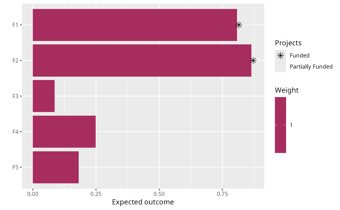
# plot solution
plot(p1, s1)
 # build another problem that includes feature weights
p2 <- p1 %>% add_feature_weights("weight")
# solve problem with feature weights
s2 <- solve(p2)
#> Set parameter Username
#> Set parameter LicenseID to value 2806834
#> Set parameter TimeLimit to value 2147483647
#> Set parameter MIPGap to value 0
#> Set parameter ScaleFlag to value 2
#> Set parameter NumericFocus to value 1
#> Set parameter Presolve to value 2
#> Set parameter Threads to value 1
#> Set parameter PoolSolutions to value 1
#> Set parameter PoolSearchMode to value 2
#> Academic license - for non-commercial use only - expires 2027-04-14
#> Gurobi Optimizer version 13.0.1 build v13.0.1rc0 (linux64 - "Ubuntu 24.04.2 LTS")
#>
#> CPU model: 11th Gen Intel(R) Core(TM) i7-1185G7 @ 3.00GHz, instruction set [SSE2|AVX|AVX2|AVX512]
#> Thread count: 4 physical cores, 8 logical processors, using up to 1 threads
#>
#> Non-default parameters:
#> TimeLimit 2147483647
#> MIPGap 0
#> ScaleFlag 2
#> NumericFocus 1
#> Presolve 2
#> Threads 1
#> PoolSolutions 1
#> PoolSearchMode 2
#>
#> Optimize a model with 27 rows, 27 columns and 62 nonzeros (Max)
#> Model fingerprint: 0x641970bf
#> Model has 5 linear objective coefficients
#> Variable types: 5 continuous, 22 integer (22 binary)
#> Coefficient statistics:
#> Matrix range [9e-02, 1e+02]
#> Objective range [2e-01, 2e+00]
#> Bounds range [5e-01, 1e+00]
#> RHS range [1e+00, 2e+02]
#>
#> Found heuristic solution: objective 0.6654645
#> Presolve removed 16 rows and 12 columns
#> Presolve time: 0.00s
#> Presolved: 11 rows, 15 columns, 25 nonzeros
#> Variable types: 0 continuous, 15 integer (15 binary)
#> Root relaxation presolved: 11 rows, 15 columns, 25 nonzeros
#>
#>
#> Root relaxation: objective 1.511230e+00, 11 iterations, 0.00 seconds (0.00 work units)
#>
#> Nodes | Current Node | Objective Bounds | Work
#> Expl Unexpl | Obj Depth IntInf | Incumbent BestBd Gap | It/Node Time
#>
#> * 0 0 0 1.5112297 1.51123 0.00% - 0s
#>
#> Explored 1 nodes (11 simplex iterations) in 0.00 seconds (0.00 work units)
#> Thread count was 1 (of 8 available processors)
#>
#> Solution count 1: 1.51123
#> No other solutions better than 1.51123
#>
#> Optimal solution found (tolerance 0.00e+00)
#> Best objective 1.511229665304e+00, best bound 1.511229665304e+00, gap 0.0000%
# print solution based on feature weights
print(s2)
#> # A tibble: 1 × 21
#> solution status cost obj F1_action F2_action F3_action F4_action F5_action
#> <int> <chr> <dbl> <dbl> <lgl> <lgl> <lgl> <lgl> <lgl>
#> 1 1 OPTIMAL 199. 1.51 FALSE FALSE FALSE TRUE TRUE
#> # ℹ 12 more variables: baseline_action <lgl>, F1_project <lgl>,
#> # F2_project <lgl>, F3_project <lgl>, F4_project <lgl>, F5_project <lgl>,
#> # baseline_project <lgl>, F1 <dbl>, F2 <dbl>, F3 <dbl>, F4 <dbl>, F5 <dbl>
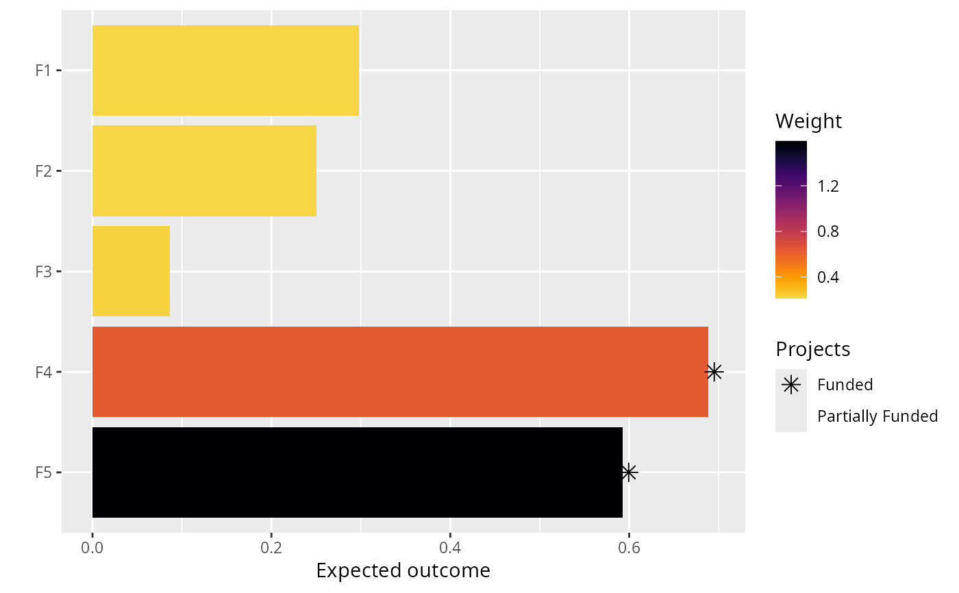
# plot solution based on feature weights
plot(p2, s2)
# build another problem that includes feature weights
p2 <- p1 %>% add_feature_weights("weight")
# solve problem with feature weights
s2 <- solve(p2)
#> Set parameter Username
#> Set parameter LicenseID to value 2806834
#> Set parameter TimeLimit to value 2147483647
#> Set parameter MIPGap to value 0
#> Set parameter ScaleFlag to value 2
#> Set parameter NumericFocus to value 1
#> Set parameter Presolve to value 2
#> Set parameter Threads to value 1
#> Set parameter PoolSolutions to value 1
#> Set parameter PoolSearchMode to value 2
#> Academic license - for non-commercial use only - expires 2027-04-14
#> Gurobi Optimizer version 13.0.1 build v13.0.1rc0 (linux64 - "Ubuntu 24.04.2 LTS")
#>
#> CPU model: 11th Gen Intel(R) Core(TM) i7-1185G7 @ 3.00GHz, instruction set [SSE2|AVX|AVX2|AVX512]
#> Thread count: 4 physical cores, 8 logical processors, using up to 1 threads
#>
#> Non-default parameters:
#> TimeLimit 2147483647
#> MIPGap 0
#> ScaleFlag 2
#> NumericFocus 1
#> Presolve 2
#> Threads 1
#> PoolSolutions 1
#> PoolSearchMode 2
#>
#> Optimize a model with 27 rows, 27 columns and 62 nonzeros (Max)
#> Model fingerprint: 0x641970bf
#> Model has 5 linear objective coefficients
#> Variable types: 5 continuous, 22 integer (22 binary)
#> Coefficient statistics:
#> Matrix range [9e-02, 1e+02]
#> Objective range [2e-01, 2e+00]
#> Bounds range [5e-01, 1e+00]
#> RHS range [1e+00, 2e+02]
#>
#> Found heuristic solution: objective 0.6654645
#> Presolve removed 16 rows and 12 columns
#> Presolve time: 0.00s
#> Presolved: 11 rows, 15 columns, 25 nonzeros
#> Variable types: 0 continuous, 15 integer (15 binary)
#> Root relaxation presolved: 11 rows, 15 columns, 25 nonzeros
#>
#>
#> Root relaxation: objective 1.511230e+00, 11 iterations, 0.00 seconds (0.00 work units)
#>
#> Nodes | Current Node | Objective Bounds | Work
#> Expl Unexpl | Obj Depth IntInf | Incumbent BestBd Gap | It/Node Time
#>
#> * 0 0 0 1.5112297 1.51123 0.00% - 0s
#>
#> Explored 1 nodes (11 simplex iterations) in 0.00 seconds (0.00 work units)
#> Thread count was 1 (of 8 available processors)
#>
#> Solution count 1: 1.51123
#> No other solutions better than 1.51123
#>
#> Optimal solution found (tolerance 0.00e+00)
#> Best objective 1.511229665304e+00, best bound 1.511229665304e+00, gap 0.0000%
# print solution based on feature weights
print(s2)
#> # A tibble: 1 × 21
#> solution status cost obj F1_action F2_action F3_action F4_action F5_action
#> <int> <chr> <dbl> <dbl> <lgl> <lgl> <lgl> <lgl> <lgl>
#> 1 1 OPTIMAL 199. 1.51 FALSE FALSE FALSE TRUE TRUE
#> # ℹ 12 more variables: baseline_action <lgl>, F1_project <lgl>,
#> # F2_project <lgl>, F3_project <lgl>, F4_project <lgl>, F5_project <lgl>,
#> # baseline_project <lgl>, F1 <dbl>, F2 <dbl>, F3 <dbl>, F4 <dbl>, F5 <dbl>
# plot solution based on feature weights
plot(p2, s2)