Add a lp_solve solver with lpSolveAPI

Add a solver to generate solutions to a project prioritization problem with the lp_solve software. This function can also be used to customize the behavior of the solver. It requires the lpSolveAPI package to be installed.

Usage

add_lpsolveapi_solver(x, gap = 0, presolve = FALSE, verbose = TRUE)

Arguments

x

problem() or multi_problem() object.

gap

numeric gap to optimality. This gap is relative and expresses the acceptable deviance from the optimal objective. For example, a value of 0.01 will result in the solver stopping when it has found a solution within 1% of optimality. Additionally, a value of 0 will result in the solver stopping when it has found an optimal solution. The default value is 0 (i.e., 0% from optimality).

presolve

logical indicating if attempts to should be made to simplify the optimization problem (TRUE) or not (FALSE). Defaults to TRUE.

verbose

logical should information be printed during optimization? Defaults to TRUE.

Value

A problem() object with the solver added to it.

Details

lp_solve is an open-source integer programming solver. Although this solver is the slowest currently supported solver, it is also the only exact algorithm solver that can be installed on all operating systems without any manual installation steps. This solver is provided so that users can try solving small project prioritization problems, without needing to install additional software. When solve moderate or large project prioritization problems, consider using add_gurobi_solver().

See also

Other solvers: add_cbc_solver(), add_default_solver(), add_gurobi_solver(), add_heuristic_solver(), add_highs_solver(), add_lpsymphony_solver(), add_random_solver(), add_rsymphony_solver()

Examples

# load data
data(sim_projects, sim_features, sim_actions)

# build problem with lpSolveAPI solver
p <-
  problem(
    sim_projects, sim_actions, sim_features,
    "name", "success", "name", "cost", "name"
  ) %>%
  add_max_wtd_sum_objective(budget = 200) %>%
  add_binary_decisions() %>%
  add_lpsolveapi_solver()

# print problem
print(p)
#> Project Prioritization Problem
#> actions:         F1_action, F2_action, F3_action, ... (6 actions)
#> projects:        F1_project, F2_project, F3_project, ... (6 projects)
#> features:        F1, F2, F3, ... (5 features)
#> action costs:    continuous values (between 0 and 103.226)
#> project success: proportion values (between 0.814 and 1)
#> objective:       maximum weighted sum objective
#> targets:         none specified
#> weights:         none specified
#> constraints:     none specified
#> decisions:       binary decision
#> solver:          lpSolveAPI solver

# solve problem
s <- solve(p)
#> 
#> Model name:  'project prioritization problem' - run #1    
#> Objective:   Maximize(R0)
#>  
#> SUBMITTED
#> Model size:       27 constraints,      27 variables,           62 non-zeros.
#> Sets:                                   0 GUB,                  0 SOS.
#>  
#> Using DUAL simplex for phase 1 and PRIMAL simplex for phase 2.
#> The primal and dual simplex pricing strategy set to 'Devex'.
#>  
#> 
#> Relaxed solution       2.21077983146 after         27 iter is B&B base.
#>  
#> Feasible solution      1.91490153549 after         36 iter,         8 nodes (gap 9.2%)
#> Improved solution       2.0146497578 after         40 iter,        11 nodes (gap 6.1%)
#> Improved solution      2.19038073725 after         52 iter,        20 nodes (gap 0.6%)
#>  
#> Optimal solution       2.19038073725 after         52 iter,        20 nodes (gap 0.6%).
#> 
#> Excellent numeric accuracy ||*|| = 7.68052e-13
#> 
#>  MEMO: lp_solve version 5.5.2.0 for 64 bit OS, with 64 bit LPSREAL variables.
#>       In the total iteration count 52, 7 (13.5%) were bound flips.
#>       There were 11 refactorizations, 0 triggered by time and 1 by density.
#>        ... on average 4.1 major pivots per refactorization.
#>       The largest [LUSOL v2.2.1.0] fact(B) had 64 NZ entries, 1.0x largest basis.
#>       The maximum B&B level was 6, 0.1x MIP order, 4 at the optimal solution.
#>       The constraint matrix inf-norm is 103.226, with a dynamic range of 1193.9.
#>       Time to load data was 0.000 seconds, presolve used 0.000 seconds,
#>        ... 0.000 seconds in simplex solver, in total 0.000 seconds.

# print solution
print(s)
#> # A tibble: 1 × 21
#>   solution status   cost   obj F1_action F2_action F3_action F4_action F5_action
#>      <int> <chr>   <dbl> <dbl> <lgl>     <lgl>     <lgl>     <lgl>     <lgl>    
#> 1        1 optima…  195.  2.19 TRUE      TRUE      FALSE     FALSE     FALSE    
#> # ℹ 12 more variables: baseline_action <lgl>, F1_project <lgl>,
#> #   F2_project <lgl>, F3_project <lgl>, F4_project <lgl>, F5_project <lgl>,
#> #   baseline_project <lgl>, F1 <dbl>, F2 <dbl>, F3 <dbl>, F4 <dbl>, F5 <dbl>

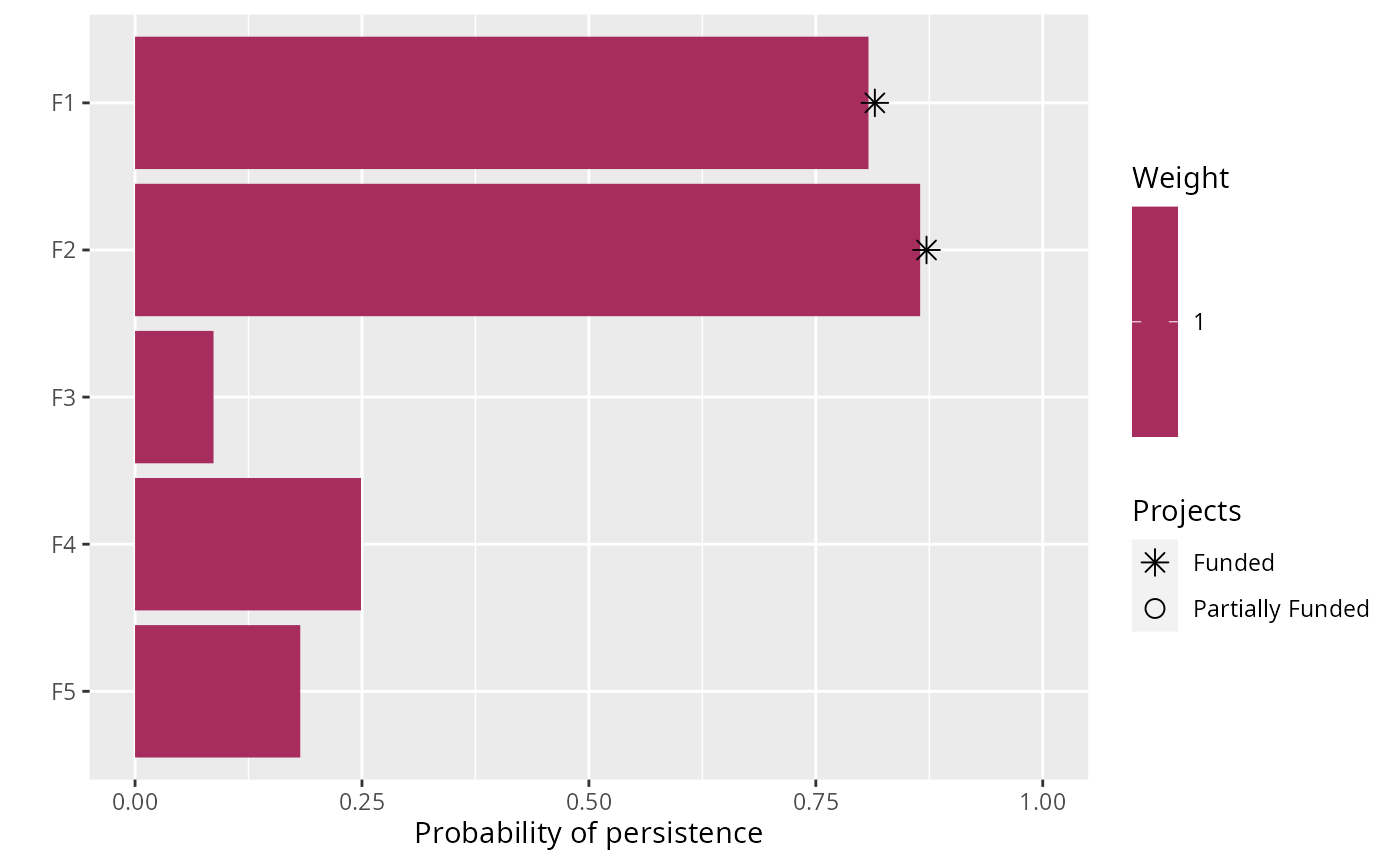
# plot solution
plot(p, s)