Plot a solution to a project prioritization problem

Create a plot to visualize how well a solution to a project prioritization problem() will maintain biodiversity.

Usage

# S3 method for class 'ProjectProblem'
plot(x, solution, n = 1, symbol_hjust = 0.007, return_data = FALSE, ...)

Arguments

x

problem() or multi_problem() object.

solution

base::data.frame() or tibble::tibble() containing the solutions. Here, rows correspond to different solutions and columns correspond to different actions. Each column in the argument to solution should be named according to a different action in x. Cell values indicate if an action is funded in a given solution or not, and should be either zero or one. Arguments to solution can contain additional columns, though they will be ignored.

n

integer solution number to visualize. Since each row in the argument to solutions corresponds to a different solution, this argument should correspond to a row in the argument to solutions. Defaults to 1.

symbol_hjust

numeric horizontal adjustment parameter to manually align the asterisks and dashes in the plot. Defaults to 0.007. Increasing this parameter will shift the symbols further right. Please note that this parameter may require some tweaking to produce visually appealing publication quality plots.

return_data

logical should the underlying data used to create the plot be returned instead of the plot? Defaults to FALSE.

...

not used.

Value

A ggplot2::ggplot() object. If return_data = TRUE, then a data.frame is returned.

Details

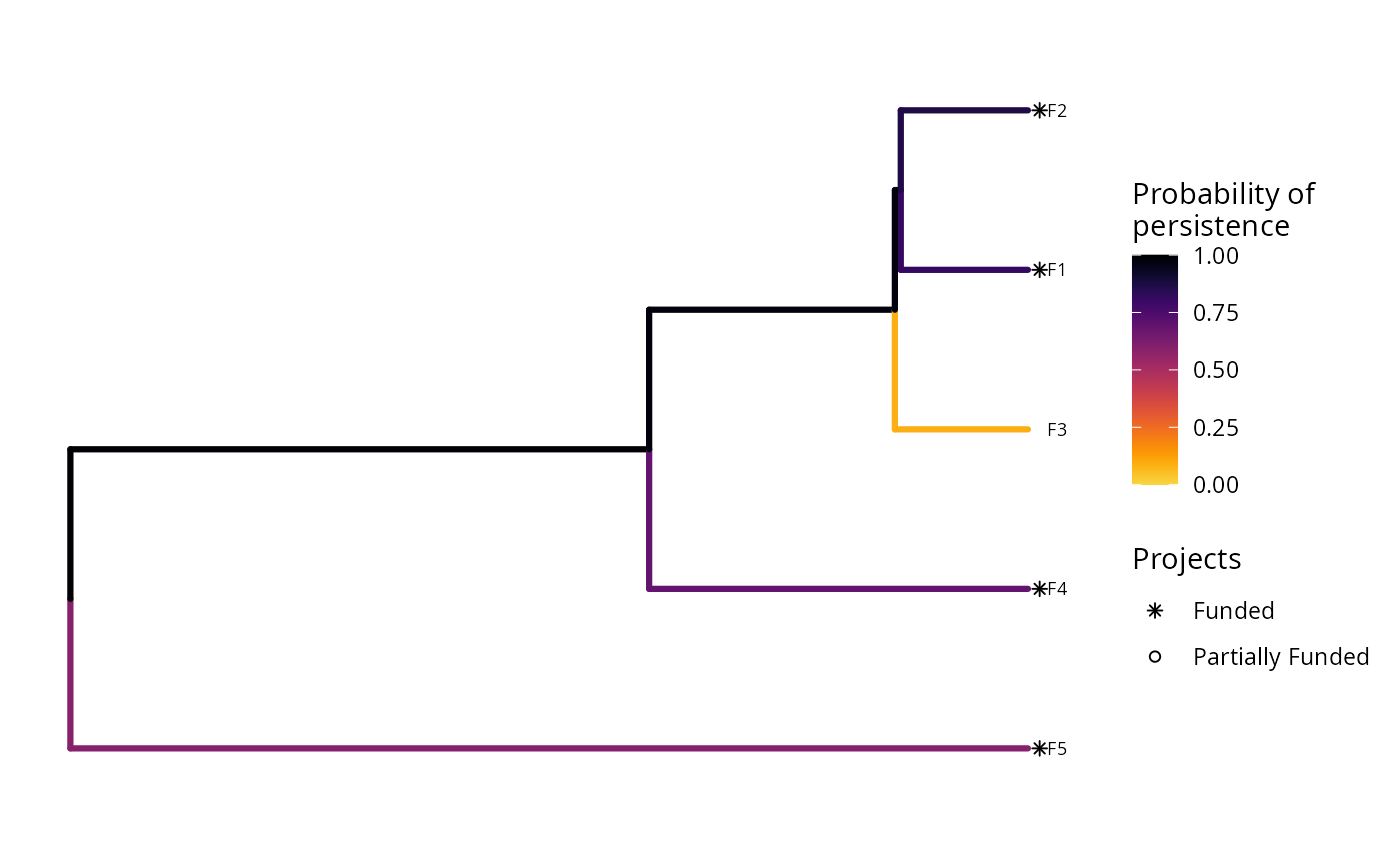
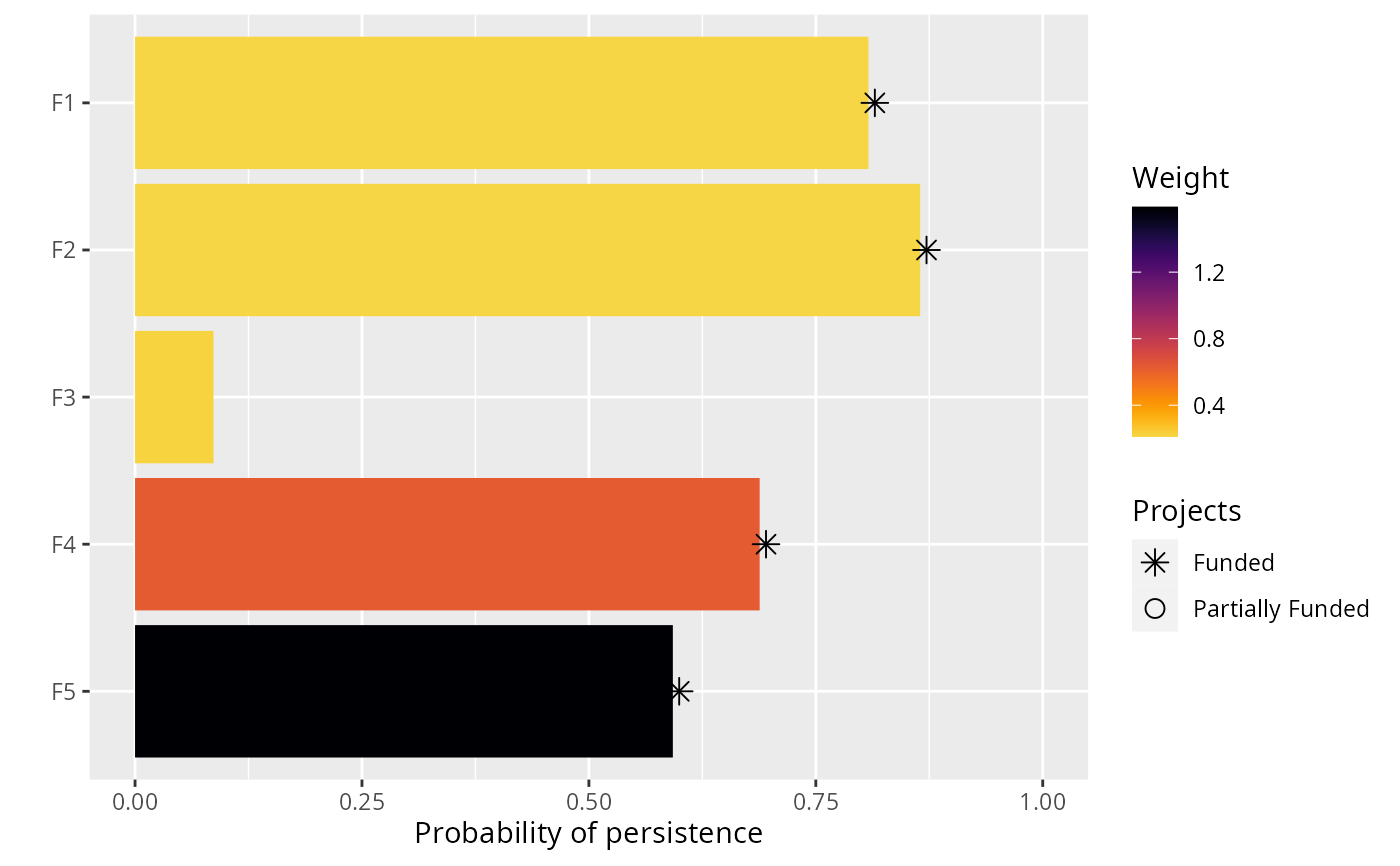
The type of plot that this function creates depends on the problem objective. If the problem objective contains phylogenetic data, then this function plots a phylogenetic tree where each branch is colored according to its probability of persistence based on the projects selected for funding by the solution. Otherwise, if the problem does not contain phylogenetic data, then this function creates a bar plot where each bar corresponds to a different feature. The height of the bars indicate the expected outcome for each feature based on the projects selected for funding by the solution, and the color of the bars indicate each feature's weight. Additionally, regardless of the problem objective, features that directly benefit from at least a single completely funded project with a non-zero cost are depicted with an asterisk symbol. Additionally, features that indirectly benefit from funded projects – because they are associated with partially funded projects that have non-zero costs and share actions with at least one funded project – are depicted with an open circle symbol.

See also

This function is a wrapper for plot_solution_phylogram() and plot_solution_barplot(), so refer to the documentation for these functions for more information.

Examples

# load data
data(sim_projects, sim_features, sim_actions)

# build problem without phylogenetic data
p1 <-
  problem(
    sim_projects, sim_actions, sim_features,
    "name", "success", "name", "cost", "name"
  ) %>%
  add_max_wtd_sum_objective(budget = 400) %>%
  add_feature_weights("weight") %>%
  add_binary_decisions()

# solve problem without phylogenetic data
s1 <- solve(p1)
#> Set parameter Username
#> Set parameter LicenseID to value 2806834
#> Set parameter TimeLimit to value 2147483647
#> Set parameter MIPGap to value 0
#> Set parameter ScaleFlag to value 2
#> Set parameter NumericFocus to value 1
#> Set parameter Presolve to value 2
#> Set parameter Threads to value 1
#> Set parameter PoolSolutions to value 1
#> Set parameter PoolSearchMode to value 2
#> Academic license - for non-commercial use only - expires 2027-04-14
#> Gurobi Optimizer version 13.0.1 build v13.0.1rc0 (linux64 - "Ubuntu 24.04.2 LTS")
#> 
#> CPU model: 11th Gen Intel(R) Core(TM) i7-1185G7 @ 3.00GHz, instruction set [SSE2|AVX|AVX2|AVX512]
#> Thread count: 4 physical cores, 8 logical processors, using up to 1 threads
#> 
#> Non-default parameters:
#> TimeLimit  2147483647
#> MIPGap  0
#> ScaleFlag  2
#> NumericFocus  1
#> Presolve  2
#> Threads  1
#> PoolSolutions  1
#> PoolSearchMode  2
#> 
#> Optimize a model with 27 rows, 27 columns and 62 nonzeros (Max)
#> Model fingerprint: 0x85f2486a
#> Model has 5 linear objective coefficients
#> Variable types: 5 continuous, 22 integer (22 binary)
#> Coefficient statistics:
#>   Matrix range     [9e-02, 1e+02]
#>   Objective range  [2e-01, 2e+00]
#>   Bounds range     [5e-01, 1e+00]
#>   RHS range        [1e+00, 4e+02]
#> 
#> Found heuristic solution: objective 0.6654645
#> Presolve removed 16 rows and 12 columns
#> Presolve time: 0.00s
#> Presolved: 11 rows, 15 columns, 24 nonzeros
#> Variable types: 0 continuous, 15 integer (15 binary)
#> Root relaxation presolved: 11 rows, 15 columns, 24 nonzeros
#> 
#> 
#> Root relaxation: objective 1.749045e+00, 11 iterations, 0.00 seconds (0.00 work units)
#> 
#>     Nodes    |    Current Node    |     Objective Bounds      |     Work
#>  Expl Unexpl |  Obj  Depth IntInf | Incumbent    BestBd   Gap | It/Node Time
#> 
#> *    0     0               0       1.7490448    1.74904  0.00%     -    0s
#> 
#> Explored 1 nodes (11 simplex iterations) in 0.00 seconds (0.00 work units)
#> Thread count was 1 (of 8 available processors)
#> 
#> Solution count 1: 1.74904 
#> No other solutions better than 1.74904
#> 
#> Optimal solution found (tolerance 0.00e+00)
#> Best objective 1.749044775334e+00, best bound 1.749044775334e+00, gap 0.0000%

# visualize solution without phylogenetic data
plot(p1, s1)


# build problem with phylogenetic data
p2 <-
  problem(
    sim_projects, sim_actions, sim_features,
    "name", "success", "name", "cost", "name"
  ) %>%
  add_max_phylo_div_objective(budget = 400, sim_tree) %>%
  add_binary_decisions()

# solve problem with phylogenetic data
s2 <- solve(p2)
#> Set parameter Username
#> Set parameter LicenseID to value 2806834
#> Set parameter TimeLimit to value 2147483647
#> Set parameter MIPGap to value 0
#> Set parameter ScaleFlag to value 2
#> Set parameter NumericFocus to value 1
#> Set parameter Presolve to value 2
#> Set parameter Threads to value 1
#> Set parameter PoolSolutions to value 1
#> Set parameter PoolSearchMode to value 2
#> Academic license - for non-commercial use only - expires 2027-04-14
#> Gurobi Optimizer version 13.0.1 build v13.0.1rc0 (linux64 - "Ubuntu 24.04.2 LTS")
#> 
#> CPU model: 11th Gen Intel(R) Core(TM) i7-1185G7 @ 3.00GHz, instruction set [SSE2|AVX|AVX2|AVX512]
#> Thread count: 4 physical cores, 8 logical processors, using up to 1 threads
#> 
#> Non-default parameters:
#> TimeLimit  2147483647
#> MIPGap  0
#> ScaleFlag  2
#> NumericFocus  1
#> Presolve  2
#> Threads  1
#> PoolSolutions  1
#> PoolSearchMode  2
#> 
#> Optimize a model with 30 rows, 30 columns and 83 nonzeros (Max)
#> Model fingerprint: 0x6415d334
#> Model has 5 linear objective coefficients
#> Model has 3 piecewise-linear objective terms
#> Variable types: 8 continuous, 22 integer (22 binary)
#> Coefficient statistics:
#>   Matrix range     [9e-02, 1e+02]
#>   Objective range  [2e-01, 2e+00]
#>   Bounds range     [1e+00, 1e+00]
#>   RHS range        [1e+00, 4e+02]
#>   PWLObj x range   [7e-01, 5e+00]
#>   PWLObj obj range [5e-03, 1e+00]
#> 
#> Found heuristic solution: objective 1.7230322
#> Presolve removed 16 rows and 12 columns
#> Presolve time: 0.00s
#> Presolved: 17 rows, 312 columns, 333 nonzeros
#> Variable types: 297 continuous, 15 integer (15 binary)
#> Root relaxation presolved: 14 rows, 309 columns, 327 nonzeros
#> 
#> 
#> Root relaxation: objective 3.112324e+00, 13 iterations, 0.00 seconds (0.00 work units)
#> 
#>     Nodes    |    Current Node    |     Objective Bounds      |     Work
#>  Expl Unexpl |  Obj  Depth IntInf | Incumbent    BestBd   Gap | It/Node Time
#> 
#> *    0     0               0       3.1123237    3.11232  0.00%     -    0s
#> 
#> Explored 1 nodes (13 simplex iterations) in 0.01 seconds (0.00 work units)
#> Thread count was 1 (of 8 available processors)
#> 
#> Solution count 1: 3.11232 
#> No other solutions better than 3.11232
#> 
#> Optimal solution found (tolerance 0.00e+00)
#> Best objective 3.112323732332e+00, best bound 3.112323732332e+00, gap 0.0000%

# visualize solution with phylogenetic data
plot(p2, s2)