Introduction
Area of Habitat (AOH) maps aim to delineate the spatial distribution
of suitable habitat for a species (Brooks et
al. 2019). They are used to assess performance of protected
area systems, measure impacts of threats to biodiversity, and identify
priorities for conservation actions (Tracewski
et al. 2016; Rondinini et al. 2005; Durán et
al. 2020). These maps are generally produced by obtaining
geographic range data for a species, and then removing areas that do not
contain suitable habitat or occur outside the known elevational limits
for the species (Brooks et al.
2019). To help make these maps accessible, the aoh R
package provides routines for automatically creating Area of Habitat
data based on the International
Union for Conservation of Nature (IUCN) Red List of Threatened
Species. After manually downloading species range data from the IUCN
Red List, users can import them (using
read_spp_range_data()), prepare them and collate additional
information for subsequent processing (using
create_spp_info_data()), and then create Area of Habitat
data (using create_spp_aoh_data()). Global elevation and
habitat classification data are automatically downloaded (Robinson et al. 2014; Jung et al.
2020; Lumbierres et al. 2021), and data on species’
habitat preferences and elevational limits are obtained automatically
using the IUCN Red List API.
Since accessing the IUCN Red List requires a token, users may need to obtain a token and update their
R configuration to recognize the token (see README for
details).
Tutorial
Here we provide a tutorial for using the aoh R package. In this tutorial, we will generate Area of Habitat data for the following Iberian species: Pyrenean brook salamander (Calotriton asper), Iberian frog (Rana iberica), western spadefoot toad (Pelobates cultripes), and golden striped salamnader (Chioglossa lusitanica). To start off, we will load the package. We will also load the rappdirs R package to cache data, and the terra and ggplot2 R packages to visualize results.
Now we will import range data for the species. Although users would typically obtain range data from the International Union for Conservation of Nature (IUCN) Red List of Threatened Species, here we will use built-in species range data that distributed with the package for convenience. Please note that these data were not obtained from the IUCN Red List, and were manually generated using occurrence records from the Global Biodiversity Information Facility.
# find file path for data
path <- system.file("extdata", "EXAMPLE_SPECIES.zip", package = "aoh")

# import data
spp_range_data <- read_spp_range_data(path)

# preview data
print(spp_range_data)
## Simple feature collection with 4 features and 26 fields
## Geometry type: POLYGON
## Dimension: XY
## Bounding box: xmin: -9.479736 ymin: 36.59422 xmax: 3.302702 ymax: 43.76455
## Geodetic CRS: WGS 84
## # A tibble: 4 × 27
## id_no binomial presence origin seasonal compiler yrcompiled citation
## <dbl> <chr> <int> <int> <int> <chr> <dbl> <chr>
## 1 979 Alytes dickhilleni 1 1 1 Derived… NA NA
## 2 59448 Calotriton asper 1 1 1 Derived… NA NA
## 3 4657 Chioglossa lusita… 1 1 1 Derived… NA NA
## 4 58622 Rana iberica 1 1 1 Derived… NA NA
## # ℹ 19 more variables: subspecies <chr>, subpop <chr>, source <chr>,
## # island <chr>, tax_comm <chr>, dist_comm <chr>, generalisd <int>,
## # legend <chr>, kingdom <chr>, phylum <chr>, class <chr>, order_ <chr>,
## # family <chr>, genus <chr>, category <chr>, marine <chr>, terrestial <chr>,
## # freshwater <chr>, geometry <POLYGON [°]>Next, we will prepare all the range data for generating Area of Habitat data. This procedure – in addition to repairing any geometry issues in the spatial data – will obtain information on the species’ habitat preferences and elevational limits (via the IUCN Red List of Threatened Species). We also specify a folder to cache the downloaded data so that we won’t need to re-download it again during subsequent runs.
# specify cache directory
cache_dir <- user_data_dir("aoh")

# create cache_dir if needed
if (!file.exists(cache_dir)) {
  dir.create(cache_dir, showWarnings = FALSE, recursive = TRUE)
}

# prepare information
spp_info_data <- create_spp_info_data(spp_range_data, cache_dir = cache_dir)
We can now generate Area of Habitat data for the species. By default, these data will be generated using elevation data derived from Robinson et al. (2014) and habitat data derived from Lumbierres et al. (2021). Similar to before, we also specify a folder to cache the downloaded datasets so that we won’t need to re-downloaded again during subsequent runs.
# specify cache directory
cache_dir <- user_data_dir("aoh")

# specify folder to save Area of Habitat data
## although we use a temporary directory here to avoid polluting your computer
## with examples files, you would normally specify the folder
## on your computer where you want to save data
output_dir <- tempdir()

# generate Area of Habitat data
## note that this function might take a complete because it will need to
## download the global habitat and elevation data that first time you run it.
spp_aoh_data <- create_spp_aoh_data(
  spp_info_data, output_dir = output_dir, cache_dir = cache_dir
)
While running the code, we see that it displayed a message telling us
that certain habitat classes were not available (i.e.,
"7.1", "7.2"). This is fine. It is not
an error. The reason we see this message is because although
the global habitat dataset contains the majority of IUCN
habitat classes for terrestrial environments, it does not contain
every single IUCN habitat class (see Lumbierres
et al. 2021 for details). Upon checking the IUCN
habitat classes, we can see that these classes correspond to
artificial aquatic areas and also caves and other subterranean
environments. Although failing to account for such habitats could
potentially be an issue, here we will assume that accounting for the
species’ non-subterranean habitats is sufficient to describe their
spatial distribution (Ficetola et al.
2014).
# preview results
## resulting dataset is a simple features (sf) object containing
## spatial geometries for cleaned versions of the range data
## (in the geometry column) and the following additional columns:
##
## - id_no            : IUCN Red List taxon identifier
## - seasonal         : integer identifier for seasonal distributions
## - category         : character IUCN Red List threat category
## - full_habitat_code: All IUCN Red List codes for suitable habitat classes
##                      (multiple codes are delimited using "|" symbols)
## - habitat_code     : IUCN Red List codes for suitable habitat classes
##                      used to create AOH maps
## - elevation_lower  : lower limit for the species on IUCN Red List
## - elevation_upper  : upper limit for the species on IUCN Red List
## - xmin             : minimum x-coordinate for Area of Habitat data
## - xmax             : maximum x-coordinate for Area of Habitat data
## - ymin             : minimum y-coordinate for Area of Habitat data
## - ymax             : maximum y-coordinate for Area of Habitat data
## - path             : file path for Area of Habitat data (GeoTIFF format)
##
## since data obtained from the IUCN Red List cannot be redistributed,
## we will only show some of the columns in this object
##
## N.B., you can view all columns on your computer with:
##> print(spp_aoh_data, width = Inf)
print(spp_aoh_data[, c("id_no", "binomial", "seasonal", "path")])
## Simple feature collection with 4 features and 4 fields
## Geometry type: POLYGON
## Dimension: XY
## Bounding box: xmin: -914664.9 ymin: 4364387 xmax: 318665.2 ymax: 5066721
## Projected CRS: World_Behrmann
## # A tibble: 4 × 5
## id_no binomial seasonal path geometry
## <dbl> <chr> <int> <chr> <POLYGON [m]>
## 1 979 Alytes dickhilleni 1 /tmp/Rtmp3McxI… ((-105506.8 4465112, -10…
## 2 59448 Calotriton asper 1 /tmp/Rtmp3McxI… ((-238681 5029057, -2377…
## 3 4657 Chioglossa lusitanica 1 /tmp/Rtmp3McxI… ((-859201.6 4559278, -85…
## 4 58622 Rana iberica 1 /tmp/Rtmp3McxI… ((-849801.9 4614149, -84…After generating the Area of Habitat data, we can import them.
# import the Area of Habitat data
## since the data for each species have a different spatial extent
## (to reduce file sizes), we will import each dataset separately in a list
spp_aoh_rasters <- lapply(spp_aoh_data$path, rast)

# preview raster data
print(spp_aoh_rasters)
## [[1]]
## class : SpatRaster
## size : 2593, 3701, 1 (nrow, ncol, nlyr)
## resolution : 100, 100 (x, y)
## extent : -467931, -97831, 4364377, 4623677 (xmin, xmax, ymin, ymax)
## coord. ref. : World_Behrmann
## source : 979_1.tif
## name : lyr1
## min value : 0
## max value : 1
##
## [[2]]
## class : SpatRaster
## size : 2266, 5670, 1 (nrow, ncol, nlyr)
## resolution : 100, 100 (x, y)
## extent : -248331, 318669, 4838277, 5064877 (xmin, xmax, ymin, ymax)
## coord. ref. : World_Behrmann
## source : 59448_1.tif
## name : lyr1
## min value : 0
## max value : 1
##
## [[3]]
## class : SpatRaster
## size : 5149, 5361, 1 (nrow, ncol, nlyr)
## resolution : 100, 100 (x, y)
## extent : -914731, -378631, 4551877, 5066777 (xmin, xmax, ymin, ymax)
## coord. ref. : World_Behrmann
## source : 4657_1.tif
## name : lyr1
## min value : 0
## max value : 1
##
## [[4]]
## class : SpatRaster
## size : 4978, 7512, 1 (nrow, ncol, nlyr)
## resolution : 100, 100 (x, y)
## extent : -904331, -153131, 4568977, 5066777 (xmin, xmax, ymin, ymax)
## coord. ref. : World_Behrmann
## source : 58622_1.tif
## name : lyr1
## min value : 0
## max value : 1We can see that the Area of Habitat data for each species are stored
in separate spatial (raster) datasets with different extents. Although
this is useful because it drastically reduces the total size of the data
for each species, it can make it difficult to work with data for
multiple species. To address this, we can use the
terra_combine() function to automatically align and combine
the spatial data for all species’ distributions into a single spatial
dataset.
# combine raster data
spp_aoh_rasters <- terra_combine(spp_aoh_rasters)

# assign identifiers to layer names
names(spp_aoh_rasters) <- paste0(
  "AOH_", spp_aoh_data$id_no, "_", spp_aoh_data$seasonal
)

# preview raster data
print(spp_aoh_rasters)
## class : SpatRaster
## size : 7024, 12334, 4 (nrow, ncol, nlyr)
## resolution : 100, 100 (x, y)
## extent : -914731, 318669, 4364377, 5066777 (xmin, xmax, ymin, ymax)
## coord. ref. : World_Behrmann
## source(s) : memory
## varnames : 979_1
## 59448_1
## 4657_1
## ...
## names : AOH_979_1, AOH_59448_1, AOH_4657_1, AOH_58622_1
## min values : 0, 0, 0, 0
## max values : 1, 1, 1, 1Finally, let’s create some maps to compare the range data with the Area of habitat data. Although we could create these maps manually (e.g., using the ggplot2 R package), we will use a plotting function distributed with the aoh R package for convenience.
# create maps
## N.B. you might need to install the ggmap package to create the maps
map <-
  plot_spp_aoh_data(
    spp_aoh_data,
    zoom = 6,
    maptype = "stamen_toner_background"
  ) +
  scale_fill_viridis_d() +
  scale_color_manual(values = c("range" = "red")) +
  scale_size_manual(values = c("range" = 0.5)) +
  theme(
    axis.title = element_blank(),
    axis.text = element_text(size = 6),
    strip.text = element_text(color = "white"),
    strip.background = element_rect(fill = "black", color = "black")
  )

# display maps
print(map)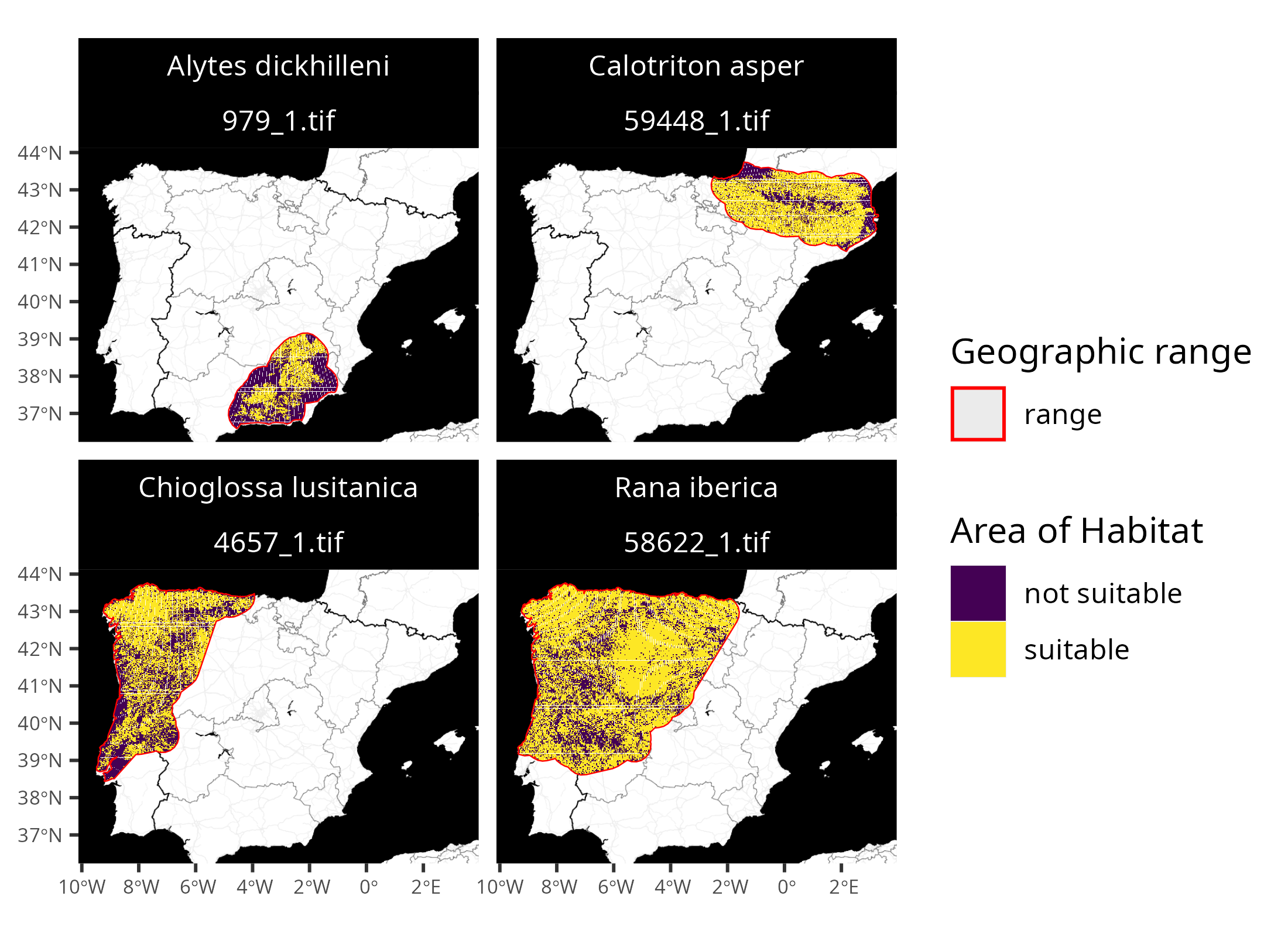
Frequently asked questions
Here we provide answers to some of the frequently asked questions encountered when using the package.
-
I see the following error message
Error : need an API key for Red List data, how do I resolve this?This error message indicates that you need to obtain a token to access the IUCN Red List API, or that you need to complete the setup process so that R can use the token. For further details on resolving this issue, please see below for details on obtaining access to the IUCN Red List API. If you have previously completed the set up procedures and still receive this error message, please try completing them again.
-
How do I obtain access to the IUCN Red List API?
You will need to obtain a token to access the IUCN Red List API (if you do not have one already). To achieve this, please visit the IUCN API website (https://api.iucnredlist.org/), click the “Generate a token” link at the top of the web page, and fill out the form to apply for a token. You should then receive a token shortly after completing the form (but not immediately). After receiving a token, you will need to complete some additional steps so that R can use this token to access the IUCN Red List API.
Please open the
.Renvironfile on your computer (e.g., usingusethis::edit_r_environ()). Next, please add the following text to the file (replacing the string with the token) and save the file:IUCN_REDLIST_KEY="your_actual_token_not_this_string"Please restart your R session. You should now be able to access the IUCN Red List API. To verify this, please try running the following R code and – assuming everything works correctly – you should see the current version of the IUCN Red List:
# verify access to IUCN Red List API
rredlist::rl_version()
If these instructions did not work, please consult the documentation for the rredlist R package for further details.
-
Where can I find species range data for generating Area of Habitat data?
Species range data can be obtained from the IUCN Red List (see Spatial Data Download resources). They can also be obtained from other data sources (see the question below for details).
-
I keep seeing this message
Error in x$.self$finalize() : attempt to apply non-function, what does it mean?This message is commonly encountered when using the terra package with large datasets. Although there is currently no known solution to prevent this message from appearing, the message can be safely ignored (see here for details). This is because the message does not stop R from completing spatial data processing – meaning that R will continue processing data even when this message is displayed – and the underlying cause of the message is not thought to result in incorrect calculations.
-
Can I produce Area of Habitat data for thousands of species globally?
Yes, the package can generate Area of Habitat data for all terrestrial amphibians, mammals, birds, and reptiles. To accomplish this, you will need a system with at least 16 Gb RAM and 65 Gb disk space. The processing could take a couple of days (e.g., if processing all amphibian species) or weeks (e.g., if processing all bird species) to complete. An example script for processing global data is available on the online code repository (see here). Additionally, since a lot of memory is required to process data for all bird species globally, it is recommended to split the full dataset containing all bird species into multiple chunks (e.g., six chunks) and process each of these chunks separately.
-
How can I speed up the processing for Area of Habitat data?
The
create_spp_aoh_data()function can use different software engines for data processing (specified via theengineparameter). Although each engine produces the same results, some engines are more computationally efficient than others. The default"terra"engine uses the terra package for processing. Although this engine is easy to install and fast for small datasets, it does not scale well for larger datasets. It is generally recommended to use the"gdal"engine in all cases where possible. Although the"gdal"engine requires installation of additional software (see the package README for instructions), it is much faster than the other engines. Additionally, the"grass"engine is also available. This engine can be faster than the"terra"engine when processing many species across large spatial extents. However, benchmarks indicate that it is slower than the"gdal"engine. -
Can I use species range data from other data sources (instead of the IUCN Red List)?
Yes, you can use species range data from a variety of sources. For example, species range data could be obtained from governmental (e.g., data for federally listed species in Canada are available through the Government of Canada data portal) and non-governmental organizations (e.g., Botanical Information and Ecology Network and Map of Life). These data can also be produced using observation records (e.g., following Palacio et al. 2021) from data repositories (e.g., Global Biodiversity Information Facility and Atlas of Living Australia). After obtaining species range data, they will need to be formatted so that they follow the data format conventions used by the IUCN Red List. This means that the species range data must contain the following columns:
id_no,presence,origin,seasonal,terrestrial(orterrestial),freshwater, andmarine. For further details on what values these columns should contain, please see the Species range data format section in the documentation forcreate_spp_info_data()and the IUCN Red List documentation. Additionally, note that if you wish to use the IUCN Red List for specifying habitat preference data, please ensure that theid_nospecified for each species follows the taxon identifiers used by the IUCN Red List. For example, the tutorial used manually generated species range data for the Pyrenean brook salamander (Calotriton asper). To ensure that correct habitat preference data were obtained for this species from the the IUCN Red List, theid_novalue specified for this species was specified as59448. -
Can I use species elevational limit data from other sources?
Yes, you can use elevational limit data from other sources. For example, for birds it is important to use the “Occasional minimum altitude” and “Occasional maximum altitude” estimates for those species for which these are coded in the IUCN Red List. These data are available on request from BirdLife International (see https://datazone.birdlife.org/contact-us/request-our-data). To use such data, you will need to manually create a table containing the species’ summary information. This table will need to contain information on the species’ elevational limits, as well as their habitat preferences and threat status (see
get_spp_summary_data()for the correct format). After preparing these data, they can be used to collate the information needed for processing Area of Habitat data (viacreate_spp_info_data()) and, in turn, create Area of Habitat data (viacreate_spp_aoh_data()). -
Can I use elevation data from other data sources?
Yes, you can use elevation data from a variety of sources. For example, elevation data could be derived from NASA’s Shuttle Radar Topography Mission (SRTM). After preparing the elevation data, they can be used to create Area of Habitat data (via
create_spp_aoh_data()). For more information, see the Customization vignette. -
Can I use habitat classification data from other data sources?
Yes, you can use habitat classification data from a variety of sources. For example, the habitat classification data could be derived from Copernicus Corine Land Cover, and MODIS Land Cover data (MCD12Q1). To use such data, you will also need to develop a crosswalk table to specify which land cover (or habitat) classes correspond to which habitat classes as defined by the IUCN Red List Habitat Classification Scheme (e.g., see Tracewski et al. 2016; Lumbierres et al. 2021). After preparing the habitat classification data and the crosswalk table, they can be used to create Area of Habitat data (via
create_spp_aoh_data()). For more information, see the Customization vignette. -
The output Area of Habitat data have different spatial extents, how can I combine them together?
The
terra_combine()function can be used to align and combine alistof rasterterra::rast()objects into a single object. Note that this procedure is only recommended when all species occur in the same geographic region. Please see the tutorial above for an example of using this function to combine Area of Habitat data for multiple species into a single object.
Conclusion
Hopefully, this vignette has provided a useful introduction to the package. If you encounter any issues when running the code in this tutorial – or when adapting the code for your own work – please see the following section. Additionally, if you have any questions about using the package or suggestions for improving it, please file an issue at the package’s online code repository.