wdpar: Interface to the World Database on Protected Areas
Jeffrey O. Hanson
2026-01-20
Source:vignettes/wdpar.Rmd
wdpar.RmdIntroduction
Protected Planet provides the most comprehensive data for conservation areas worldwide. Specifically, it provides the World Database on Protected Areas (WDPA) and the World Database on Other Effective Area-Based Conservation Measures (WDOECM). These databases are used to monitor the performance of existing protected areas, and identify priority areas for future conservation efforts. Additionally, these databases receive monthly updates from government agencies and non-governmental organizations. However, they are associated with several issues that need to be addressed prior to analysis and the dynamic nature of these databases means that the entire data cleaning process needs to be repeated after obtaining a new version.
The wdpar R package provides an interface to data available on Protected Planet. Specifically, it can be used to automatically obtain data from the World Database on Protected Areas (WDPA) and the World Database on Other Effective Area-Based Conservation Measures (WDOECM). It also provides methods for cleaning data from these databases following best practices (outlined in Butchart et al. 2015; Protected Planet 2021; Runge et al. 2015). In this vignette, we provide a tutorial and recommendations for using the package.
Tutorial
Here we will provide a short introduction to the wdpar R package. First, we will load the wdpar R package. We will also load the dplyr and ggmap R packages to help explore the data.
Now we will download protected area data for Malta from Protected Planet. We can
achieve this by specifying Malta’s country name
(i.e. "Malta") or Malta’s ISO3 code
(i.e. "MLT"). Since data are downloaded to a temporary
directory by default, we will specify that the data should be downloaded
to a persistent directory. This means that R won’t have to re-download
the same dataset every time we restart our R session, and R can simply
re-load previously downloaded datasets as needed.
# download protected area data for Malta
# (excluding areas represented as point localities)
mlt_raw_pa_data <- wdpa_fetch(
  "Malta", wait = TRUE, download_dir = rappdirs::user_data_dir("wdpar")
)
Next, we will clean the data set. Briefly, the cleaning steps
include: excluding protected areas that are not yet implemented,
excluding protected areas with limited conservation value, replacing
missing data codes (e.g. "0") with missing data values
(i.e. NA), replacing protected areas represented as points
with circular protected areas that correspond to their reported extent,
repairing any topological issues with the geometries, and erasing
overlapping areas. Please note that, by default, spatial data processing
is performed at a scale suitable for national scale analyses (see below
for recommendations for local scale analyses). For more information on
the data cleaning procedures, see wdpa_clean().
# clean Malta data
mlt_pa_data <- wdpa_clean(mlt_raw_pa_data)
After cleaning the data set, we will perform an additional step that involves clipping the terrestrial protected areas to Malta’s coastline. Ideally, we would also clip the marine protected areas to Malta’s Exclusive Economic Zone (EEZ) but such data are not as easy to obtain on a per country basis (but see https://www.marineregions.org/eez.php)).
# download Malta boundary from Global Administrative Areas dataset
file_path <- tempfile(fileext = ".gpkg")
download.file(
  "https://geodata.ucdavis.edu/gadm/gadm4.1/gpkg/gadm41_MLT.gpkg",
  file_path
)

# import Malta's boundary
mlt_boundary_data <- sf::read_sf(file_path, "ADM_ADM_0")

# repair any geometry issues, dissolve the border, reproject to same
# coordinate system as the protected area data, and repair the geometry again
mlt_boundary_data <-
  mlt_boundary_data %>%
  st_set_precision(1000) %>%
  sf::st_make_valid() %>%
  st_set_precision(1000) %>%
  st_combine() %>%
  st_union() %>%
  st_set_precision(1000) %>%
  sf::st_make_valid() %>%
  st_transform(st_crs(mlt_pa_data)) %>%
  sf::st_make_valid()

# clip Malta's protected areas to the coastline
mlt_pa_data <-
  mlt_pa_data %>%
  filter(REALM == "Terrestrial") %>%
  st_intersection(mlt_boundary_data) %>%
  rbind(mlt_pa_data %>%
        filter(REALM == "Marine") %>%
        st_difference(mlt_boundary_data)) %>%
  rbind(mlt_pa_data %>% filter(!REALM %in% c("Terrestrial", "Marine")))
## Warning: attribute variables are assumed to be spatially constant throughout
## all geometries
## Warning: attribute variables are assumed to be spatially constant throughout
## all geometries
# recalculate the area of each protected area
mlt_pa_data <-
  mlt_pa_data %>%
  mutate(AREA_KM2 = as.numeric(st_area(.)) * 1e-6)
Now that we have finished cleaning the data, let’s preview the data. For more information on what these columns mean, please refer to the official manual (available in English, French, Spanish, and Russian).
# print first six rows of the data
head(mlt_pa_data)
## Simple feature collection with 6 features and 35 fields
## Geometry type: GEOMETRY
## Dimension: XY
## Bounding box: xmin: 1382584 ymin: 4289200 xmax: 1406320 ymax: 4298958
## Projected CRS: World_Behrmann
## # A tibble: 6 × 36
## SITE_ID SITE_PID SITE_TYPE NAME_ENG NAME DESIG DESIG_ENG DESIG_TYPE IUCN_CAT
## <int> <chr> <chr> <chr> <chr> <chr> <chr> <chr> <chr>
## 1 5.56e8 5557003… PA "Il-Pon… "Il-… Rise… Nature R… National Ia
## 2 5.56e8 5555886… PA "Il-Maj… "Il-… Park… National… National II
## 3 5.56e8 5557717… PA "L-Inħa… "L-I… Park… National… National II
## 4 1.75e5 174757 PA "Il-Ġon… "Il-… List… List of … National III
## 5 1.75e5 174758 PA "Bidnij… "Bid… List… List of … National III
## 6 1.94e5 194415 PA "Il-Ġon… "Il-… List… List of … National III
## # ℹ 27 more variables: INT_CRIT <chr>, REALM <chr>, REP_M_AREA <dbl>,
## # GIS_M_AREA <dbl>, REP_AREA <dbl>, GIS_AREA <dbl>, NO_TAKE <chr>,
## # NO_TK_AREA <dbl>, STATUS <chr>, STATUS_YR <dbl>, GOV_TYPE <chr>,
## # GOVSUBTYPE <chr>, OWN_TYPE <chr>, OWNSUBTYPE <chr>, MANG_AUTH <chr>,
## # MANG_PLAN <chr>, VERIF <chr>, METADATAID <int>, PRNT_ISO3 <chr>,
## # ISO3 <chr>, SUPP_INFO <chr>, CONS_OBJ <chr>, INLND_WTRS <chr>,
## # OECM_ASMT <chr>, GEOMETRY_TYPE <chr>, AREA_KM2 <dbl>, …We will now reproject the data to longitude/latitude coordinates (EPSG:4326) for visualization purposes.
# reproject data
mlt_pa_data <- st_transform(mlt_pa_data, 4326)
Next, we can plot a map showing the boundaries of Malta’s protected area system.
# download basemap for making the map
bg <- get_stadiamap(
  unname(st_bbox(mlt_pa_data)), zoom = 8,
  maptype = "stamen_terrain_background", force = TRUE
)

# print map
ggmap(bg) +
geom_sf(data = mlt_pa_data, fill = "#31A35480", inherit.aes = FALSE) +
theme(axis.title = element_blank())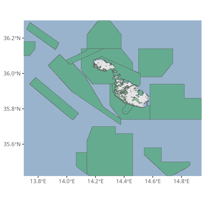
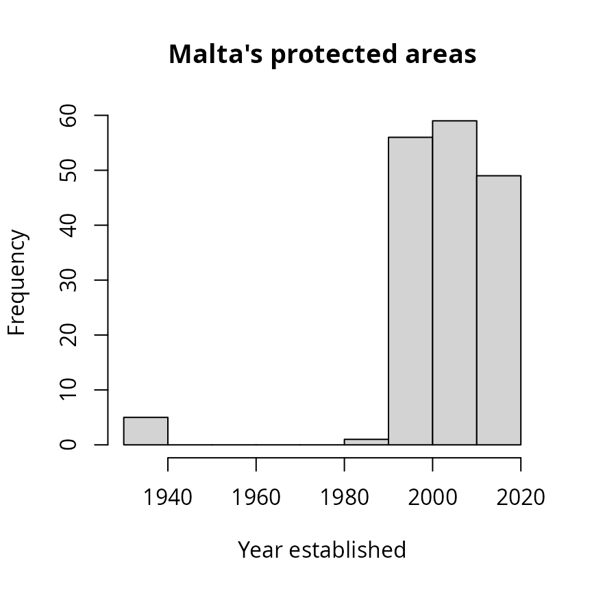
We can also create a histogram showing the year when each protected area was established.
hist(
  mlt_pa_data$STATUS_YR,
  main = "Malta's protected areas",
  xlab = "Year established"
)
Now let’s calculate some statistics. We can calculate the total amount of land and ocean inside Malta’s protected area system (km2).
# calculate total amount of area inside protected areas (km^2)
statistic <-
  mlt_pa_data %>%
  as.data.frame() %>%
  select(-geometry) %>%
  group_by(REALM) %>%
  summarize(area_km = sum(AREA_KM2)) %>%
  ungroup() %>%
  arrange(desc(area_km))

# print statistic
print(statistic)
## # A tibble: 3 × 2
## REALM area_km
## <chr> <dbl>
## 1 Marine 4523.
## 2 Terrestrial 84.0
## 3 Coastal 8.91We can also calculate the percentage of land inside its protected area system that are managed under different categories (i.e. using the protected area management categories defined by The International Union for Conservation of Nature).
# calculate percentage of land inside protected areas (km^2)
statistic <-
  mlt_pa_data %>%
  as.data.frame() %>%
  select(-geometry) %>%
  group_by(IUCN_CAT) %>%
  summarize(area_km = sum(AREA_KM2)) %>%
  ungroup() %>%
  mutate(percentage = (area_km / sum(area_km)) * 100) %>%
  arrange(desc(area_km))

# print statistic
print(statistic)
## # A tibble: 7 × 3
## IUCN_CAT area_km percentage
## <chr> <dbl> <dbl>
## 1 IV 4191. 90.8
## 2 Not Reported 390. 8.45
## 3 V 22.1 0.478
## 4 Not Assigned 8.39 0.182
## 5 II 3.39 0.0734
## 6 III 0.191 0.00414
## 7 Ia 0.101 0.00218We can also plot a map showing Malta’s protected areas and color each area according to it’s management category.
ggmap(bg) +
geom_sf(aes(fill = IUCN_CAT), data = mlt_pa_data, inherit.aes = FALSE) +
theme(axis.title = element_blank(), legend.position = "bottom")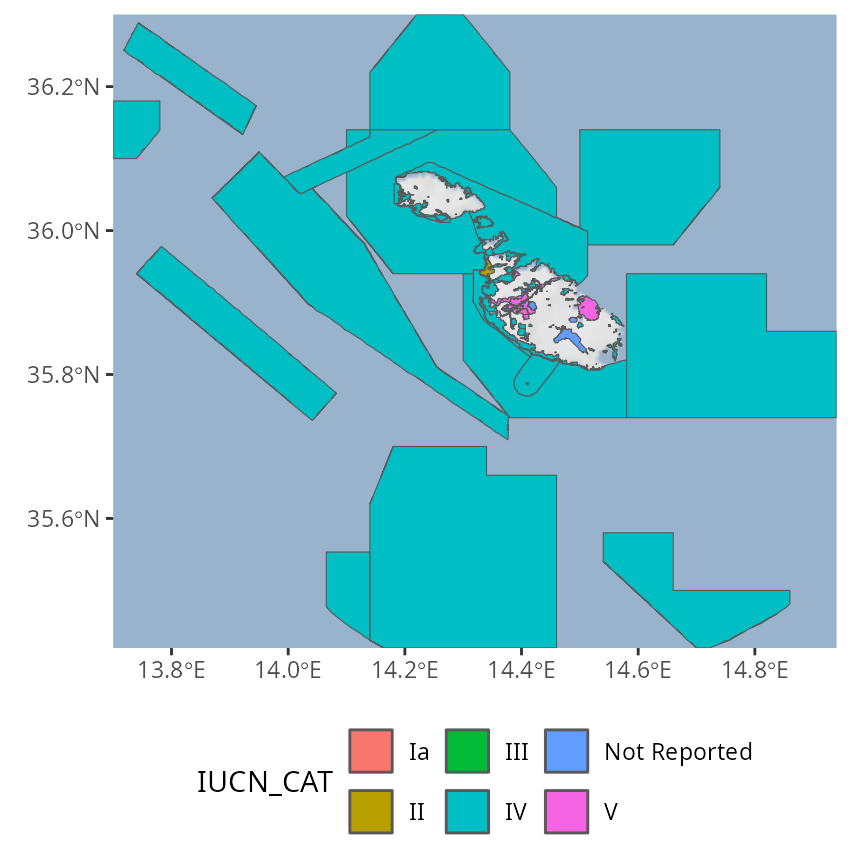
Recommended practices for large datasets
The wdpar R package can be used to clean large datasets
assuming that sufficient computational resources and time are available.
Indeed, it can clean data spanning large countries, multiple countries,
and even the full global dataset. When processing the full global
dataset, it is recommended to use a computer system with at least 32 GB
RAM available and to allow for at least one full day for the data
cleaning procedures to complete. It is also recommended to avoid using
the computer system for any other tasks while the data cleaning
procedures are being completed, because they are very computationally
intensive. Additionally, when processing large datasets – and especially
for the global dataset – it is strongly recommended to disable the
procedure for erasing overlapping areas. This is because the built-in
procedure for erasing overlaps is very time consuming when processing
many protected areas, so that information on each protected area can be
output (e.g. IUCN category, year established). Instead, when cleaning
large datasets, it is recommended to run the data cleaning procedures
with the procedure for erasing overlapping areas disabled (i.e. with
erase_overlaps = FALSE). After the data cleaning procedures
have completed, the protected area data can be manually dissolved to
remove overlapping areas (e.g. using wdpa_dissolve()). For
an example of these procedures, please see below.
# download protected area data for multiple of countries
## (i.e. Portugal, Spain, France)
raw_pa_data <-
  c("PRT", "ESP", "FRA") %>%
  lapply(wdpa_fetch, wait = TRUE,
         download_dir = rappdirs::user_data_dir("wdpar")) %>%
  bind_rows()
# clean protected area data (with procedure for erasing overlaps disabled)
full_pa_data <- wdpa_clean(raw_pa_data, erase_overlaps = FALSE)

# at this stage, the data could be filtered based on extra criteria (if needed)
## for example, we could subset the data to only include protected areas
## classified as IUCN category Ia or Ib
sub_pa_data <-
  full_pa_data %>%
  filter(IUCN_CAT %in% c("Ia", "Ib"))

# dissolve all geometries together (removing spatial overlaps)
pa_data <- wdpa_dissolve(sub_pa_data)

# preview data
print(pa_data)
## Simple feature collection with 1 feature and 1 field
## Geometry type: MULTIPOLYGON
## Dimension: XY
## Bounding box: xmin: -3274101 ymin: 3403947 xmax: 879505 ymax: 5609364
## Projected CRS: World_Behrmann
## Precision: 1500
## id geometry
## 1 1 MULTIPOLYGON (((-1747881 34...## 10302220212 [m^2]Recommended practices for local scale analyses
The default parameters for the data cleaning procedures are well
suited for national-scale analyses. Although these parameters reduce
memory requirements and the time needed to complete the data cleaning
procedures, they can produce protected area boundaries that appear
overly “blocky” – lacking smooth edges – when viewed at finer scales. As
such, it is strongly recommended to increase the level of spatial
precision when cleaning data for local scale analyses (via the
geometry_precision parameter of the
wdpa_clean() function).
Here we will explore the consequences of using the default parameters for the data cleaning procedures when working at a local scale. This will help illustrate why it can be important to adjust the spatial precision of the data cleaning procedures. To begin with, we will obtain data for a small protected area. Specifically, we will extract a protected area from the Malta dataset we downloaded earlier.
# find id for smallest reserve in cleaned dataset
mlt_reserve_id <- mlt_pa_data$SITE_ID[which.min(mlt_pa_data$AREA_KM2)]

# extract the smallest reserve from the raw dataset
mlt_raw_reserve_data <-
  mlt_raw_pa_data %>%
  filter(SITE_ID == mlt_reserve_id)

# preview data
print(mlt_raw_reserve_data)
## Simple feature collection with 1 feature and 33 fields
## Geometry type: MULTIPOLYGON
## Dimension: XY
## Bounding box: xmin: 14.24996 ymin: 36.01383 xmax: 14.25889 ymax: 36.0195
## Geodetic CRS: WGS 84
## # A tibble: 1 × 34
## SITE_ID SITE_PID SITE_TYPE NAME_ENG NAME DESIG DESIG_ENG DESIG_TYPE IUCN_CAT
## * <int> <chr> <chr> <chr> <chr> <chr> <chr> <chr> <chr>
## 1 330746 330746 PA "Ta\\' Ċ… "Ta\… Sit … Site of … National IV
## # ℹ 25 more variables: INT_CRIT <chr>, REALM <chr>, REP_M_AREA <dbl>,
## # GIS_M_AREA <dbl>, REP_AREA <dbl>, GIS_AREA <dbl>, NO_TAKE <chr>,
## # NO_TK_AREA <dbl>, STATUS <chr>, STATUS_YR <int>, GOV_TYPE <chr>,
## # GOVSUBTYPE <chr>, OWN_TYPE <chr>, OWNSUBTYPE <chr>, MANG_AUTH <chr>,
## # MANG_PLAN <chr>, VERIF <chr>, METADATAID <int>, PRNT_ISO3 <chr>,
## # ISO3 <chr>, SUPP_INFO <chr>, CONS_OBJ <chr>, INLND_WTRS <chr>,
## # OECM_ASMT <chr>, geometry <MULTIPOLYGON [°]>
# visualize data
plot(mlt_raw_reserve_data[, 1])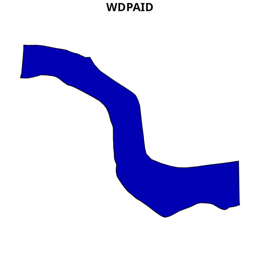
We can see that the boundary for this protected area has a high level of detail. This suggests that the protected area data is available at a resolution that is sufficient to permit local scale analyses. To help understand the consequences of cleaning data with the default parameters, we will clean this dataset using the default parameters.
# clean the data with default parameters
mlt_default_cleaned_reserve_data <- wdpa_clean(mlt_raw_reserve_data)

# preview data
print(mlt_default_cleaned_reserve_data)
## Simple feature collection with 1 feature and 35 fields
## Geometry type: POLYGON
## Dimension: XY
## Bounding box: xmin: 1375122 ymin: 4304454 xmax: 1375830 ymax: 4305007
## Projected CRS: World_Behrmann
## # A tibble: 1 × 36
## SITE_ID SITE_PID SITE_TYPE NAME_ENG NAME DESIG DESIG_ENG DESIG_TYPE IUCN_CAT
## <int> <chr> <chr> <chr> <chr> <chr> <chr> <chr> <chr>
## 1 330746 330746 PA "Ta\\' Ċ… "Ta\… Sit … Site of … National IV
## # ℹ 27 more variables: INT_CRIT <chr>, REALM <chr>, REP_M_AREA <dbl>,
## # GIS_M_AREA <dbl>, REP_AREA <dbl>, GIS_AREA <dbl>, NO_TAKE <chr>,
## # NO_TK_AREA <dbl>, STATUS <chr>, STATUS_YR <dbl>, GOV_TYPE <chr>,
## # GOVSUBTYPE <chr>, OWN_TYPE <chr>, OWNSUBTYPE <chr>, MANG_AUTH <chr>,
## # MANG_PLAN <chr>, VERIF <chr>, METADATAID <int>, PRNT_ISO3 <chr>,
## # ISO3 <chr>, SUPP_INFO <chr>, CONS_OBJ <chr>, INLND_WTRS <chr>,
## # OECM_ASMT <chr>, GEOMETRY_TYPE <chr>, AREA_KM2 <dbl>, …
# visualize data
plot(mlt_default_cleaned_reserve_data[, 1])
After cleaning the data with the default parameters, we can see that the boundary of the protected area is no longer highly detailed. For example, the smooth edges of the raw protected area data have been replaced with sharp, blocky edges. As such, subsequent analysis performed at the local scale – such as calculating the spatial extent of land cover types within this single protected area – might not be sufficiently precise. Now, let’s clean the data using parameters that are well suited for local scale analysis.
# clean the data with default parameters
mlt_fixed_cleaned_reserve_data <- wdpa_clean(
  mlt_raw_reserve_data, geometry_precision = 10000
)

# preview data
print(mlt_fixed_cleaned_reserve_data)
## Simple feature collection with 1 feature and 35 fields
## Geometry type: POLYGON
## Dimension: XY
## Bounding box: xmin: 1374929 ymin: 4304433 xmax: 1375788 ymax: 4305024
## Projected CRS: World_Behrmann
## # A tibble: 1 × 36
## SITE_ID SITE_PID SITE_TYPE NAME_ENG NAME DESIG DESIG_ENG DESIG_TYPE IUCN_CAT
## <int> <chr> <chr> <chr> <chr> <chr> <chr> <chr> <chr>
## 1 330746 330746 PA "Ta\\' Ċ… "Ta\… Sit … Site of … National IV
## # ℹ 27 more variables: INT_CRIT <chr>, REALM <chr>, REP_M_AREA <dbl>,
## # GIS_M_AREA <dbl>, REP_AREA <dbl>, GIS_AREA <dbl>, NO_TAKE <chr>,
## # NO_TK_AREA <dbl>, STATUS <chr>, STATUS_YR <dbl>, GOV_TYPE <chr>,
## # GOVSUBTYPE <chr>, OWN_TYPE <chr>, OWNSUBTYPE <chr>, MANG_AUTH <chr>,
## # MANG_PLAN <chr>, VERIF <chr>, METADATAID <int>, PRNT_ISO3 <chr>,
## # ISO3 <chr>, SUPP_INFO <chr>, CONS_OBJ <chr>, INLND_WTRS <chr>,
## # OECM_ASMT <chr>, GEOMETRY_TYPE <chr>, AREA_KM2 <dbl>, …
# visualize data
plot(mlt_fixed_cleaned_reserve_data[, 1])
Here, we specified that the spatial data processing should be
performed at a much greater level of precision (using the
geometry_precision parameter). As a consequence, we can see
– after applying the data cleaning procedures – that the protected area
boundary still retains a high level of detail. This means that the
cleaned protected area data is more suitable for local scale analysis.
If a greater level of detail is required, the level of precision could
be increased further. Note that the maximum level of detail that can be
achieved in the cleaned data is limited by the level of detail in the
raw data. This means that increasing the level of precision beyond a
certain point will have no impact on the cleaned data, because the raw
data do not provide sufficient detail for the increased precision to
alter the spatial data processing.
Additional datasets
Although the World Database on Protected Areas (WDPA) is the most comprehensive global dataset, many datasets are available for specific countries or regions that do not require such extensive data cleaning procedures. As a consequence, it is often worth looking for alternative data sets when working at smaller geographic scales before considering the World Database on Protected Areas (WDPA). The list below outlines several alternative protected area datasets and information on where they can be obtained. If you know of any such datasets that are missing, please create an issue on the GitHub repository and we can add them to the list.
- Arctic
- Australia
- The United States of America
Citation
Please cite the wdpar R package and the relevant databases in publications. To see citation details, use the code:
citation("wdpar")