Prioritize conservation projects by maximizing expected phylogenetic diversity with exact algorithms
Source:R/ppp_exact_phylo_solution.R
ppp_exact_phylo_solution.RdPrioritize funding for conservation projects with phylogenetic data and using exact algorithms. Unlike other algorithms for solving the 'Project Prioritization Protocol' (Joseph, Maloney & Possingham 2009), this method can identify solutions that are guaranteed to be optimal (or within a pre-specified optimality gap; see Underhill 1994; Rodrigues & Gaston 2002). As a consequence, it is strongly recommended to use this method for developing project prioritizations.
ppp_exact_phylo_solution(x, y, tree, budget, project_column_name,
  success_column_name, action_column_name, cost_column_name,
  locked_in_column_name = NULL, locked_out_column_name = NULL,
  gap = 1e-06, threads = 1L, number_solutions = 1L,
  time_limit = .Machine$integer.max, number_approx_points = 300,
  verbose = FALSE)
Arguments
| x |
|
|---|---|
| y |
|
| tree |
|
| budget |
|
| project_column_name |
|
| success_column_name |
|
| action_column_name |
|
| cost_column_name |
|
| locked_in_column_name |
|
| locked_out_column_name |
|
| gap |
|
| threads |
|
| number_solutions |
|
| time_limit |
|
| number_approx_points |
|
| verbose |
|
Value
A tibble object containing the
solution(s) data. Each row corresponds to a different solution, and
each column describes a different property of the solution. The object
contains a column for each project (based on the argument to
project_column_name) which contains logical values indicating
if the project was prioritized for funded (TRUE) or not
(FALSE) in a given solution. Additionally, the object also contains
the following columns:
"solution"integersolution identifier."method"charactername of method used to produce the solution(s).)"budget"numericbudget used for generating each of the of the solution(s)."obj"numericobjective value. If phylogenetic data were input, then this column contains the expected phylogenetic diversity (Faith 2008) associated with each of the solutions. Otherwise, this column contains the expected weighted species richness (i.e. the sum of the product between the species' persistence probabilities and their weights."cost"numerictotal cost associated with each of of the solution(s)."optimal"logicalindicating if each of the solution(s) is known to be optimal (TRUE) or not (FALSE). Missing values (NA) indicate that optimality is unknown (i.e. because the method used to produce the solution(s) does not provide any bounds on their quality).
Details
This function works by formulating the 'Project Prioritization Protocol' as a mixed integer programming problem (MIP) and solving it using the Gurobi optimization software suite. Although Gurobi is a commercial software, academics can obtain a special license for no cost. After downloading and installing the Gurobi software suite, the gurobi package will also need to be installed (see instructions for Linux, Mac OSX, and Windows operating systems). Finally, the gurobi package will also need to be installed (see instructions for Linux, Mac OSX, and Windows operating systems).
The objective of this problem is to maximize the amount of evolutionary history that is expected to remain within a specified period of time (e.g. 100 years; i.e. 'expected phylogenetic diversity'; Faith 2008). Let \(I\) represent the set of conservation actions (indexed by \(i\)). Let \(C_i\) denote the cost for funding action \(i\), and let \(m\) define the maximum expenditure (budget) for funding all the actions. Also, let \(S\) represent each species (indexed by \(s\)). To describe the evolutionary relationships between the species \(s \in S\), consider a phylogenetic tree that contains species \(s \in S\) with branches of known lengths. This tree can be described using mathematical notation by letting \(B\) represent the branches (indexed by \(b\)) with lengths \(L_b\) and letting \(T_{bs}\) indicate which species \(s \in S\) are associated with which phylogenetic branches \(b \in B\) using zeros and ones. Ideally, the set of species \(S\) would contain all of the species in the study area---including non-threatened species---to fully account for the benefits for funding different actions.
To guide the prioritization, the conservation actions are organized into conservation projects. Let \(J\) denote the set of conservation projects (indexed by \(j\)), and let \(A_{ij}\) denote which actions \(i \in I\) comprise each conservation project \(j \in J\) using zeros and ones. Next, let \(P_j\) represent the probability of project \(j\) being successful if it is funded. Also, let \(B_{sj}\) denote the enhanced probability that each species' \(s \in S\) associated with the project \(j \in J\) will persist if all of the actions that comprise project \(j\) are funded and that project is allocated to species \(s\).
The binary control variables \(X_i\) in this problem indicate whether each project \(i \in I\) is funded (variable equal to one) or not (variable equal to zero). The decision variables in this problem are the \(Y_{j}\), \(Z_{sj}\), \(E_s\), and \(R_b\) variables. Specifically, the binary \(Y_{j}\) variables indicate if project \(j\) is funded (variable equal to one) or not (variable equal to zero) based on which actions are funded; the binary \(Z_{sj}\) variables indicate if project \(j\) is used to manage species \(s\) (variable equal to one) or not (variable equal to zero); the semi-continuous \(E_s\) variables denote the probability that species \(s\) will go extinct; and the semi-continuous \(R_b\) variables denote the probability that phylogenetic branch \(b\) will remain in the future.
Now that we have defined all the data and variables, we can formulate the problem. For convenience, let the symbol used to denote each set also represent its cardinality (e.g. if there are ten species, let \(S\) represent the set of ten species and also the number ten).
$$ \mathrm{Maximize} \space \sum_{b = 0}^{B} L_b R_b \space \mathrm{(eqn \space 1a)} \\ \mathrm{Subject \space to} \space R_b = 1 - \prod_{s = 0}^{S} ifelse(T_{bs} == 1, \space E_s, \space 1) \space \forall \space b \in B \space \mathrm{(eqn \space 1b)} \\ E_s = 1 - \sum_{j = 0}^{J} Z_{sj} P_j B_{sj} \space \forall \space s \in S \space \mathrm{(eqn \space 1c)} \\ \sum_{i = 0}^{I} C_i \leq m \space \mathrm{(eqn \space 1d)} \\ Z_{sj} \leq Y_{j} \space \forall \space j \in J \space \mathrm{(eqn \space 1e)} \\ \sum_{j = 0}^{J} Z_{sj} = 1 \space \forall \space s \in s \space \mathrm{(eqn \space 1f)} \\ A_{ij} Y_{j} \leq X_{i} \space \forall \space i \in I, j \in J \space \mathrm{(eqn \space 1g)} \\ R_{b} \geq 0, R_{b} \leq 1 \space \forall \space b \in B \space \mathrm{(eqn \space 1h)} \\ E_{s} \geq 0, E_{s} \leq 1 \space \forall \space b \in B \space \mathrm{(eqn \space 1i)} \\ X_{i}, Y_{j}, Z_{sj} \in [0, 1] \space \forall \space i \in I, j \in J, s \in S \space \mathrm{(eqn \space 1j)} $$
The objective (eqn 1a) is to maximize the amount of expected phylogenetic history that will remain in the future. This is expressed as the sum of branch lengths (\(L_b\)) weighted by the probability that at least one of the species connected to this branch will not go extinct (\(R_b\)). Constraints (eqn 1b) state that the probability that a branch will remain (\(R_b\)) is equal to one minus the probability that all species connected to the branch will go extinct. Constraints (eqn 1c) calculate the probability that each species will go extinct according to their allocated project. Constraint (eqn 1d) ensures that the cost of all the funded actions do not exceed the budget. Constraints (eqn 1e) ensure that species can only be allocated to projects that have all of their actions funded. Constraints (eqn 1f) state that each species can only be allocated to a single project. Constraints (eqn 1g) ensure that a project cannot be funded unless all of its actions are funded. Constraints (eqns 1h, 1i) ensure that the probability variables (\(R_b\), \(E_s\)) are bounded between zero and one. Constraints (eqns 1j) ensure that the action funding (\(X_j\)), project funding (\(Y_j\)), and project allocation (\(Z_{sj}\)) variables are binary.
Although this formulation is a mixed integer quadratically constrained
programming problem (due to eqn 1b), it can be linearized and then solved
using commercial mixed integer programming solvers (e.g. Gurobi). This can
be achieved by substituting the product of the species' extinction
probabilities (eqn 1b) with the sum of the log species' extinction
probabilities and using piecewise linear approximations (described in
Hillier & Price 2005 pp. 390--392) to approximate the exponent of this term.
Although this means the problem can only be solved to a pre-specified level
of precision (controlled via the argument to number_approx_points),
advances in exact algorithm solvers mean that the problem can be solved to a
sufficient degree of precision (e.g. \(1 \times 10^{-5}\)) in a
trivial period of time.
References
Faith DP (2008) Threatened species and the potential loss of phylogenetic diversity: conservation scenarios based on estimated extinction probabilities and phylogenetic risk analysis. Conservation Biology, 22: 1461--1470.
Hillier FS & Price CC (2005) International series in operations research & management science. Springer.
Joseph LN, Maloney RF & Possingham HP (2009) Optimal allocation of resources among threatened species: A project prioritization protocol. Conservation Biology, 23, 328--338.
Rodrigues AS & Gaston KJ (2002) Optimisation in reserve selection procedures---why not? Biological Conservation, 107: 123-129.
Underhill LG (1994) Optimal and suboptimal reserve selection algorithms. Biological Conservation, 70: 85--87.
See also
For other methods for solving the 'Project Prioritization Protocol'
problem, see ppp_heuristic_phylo_solution,
ppp_manual_phylo_solution, and
ppp_random_phylo_solution.
To visualize the effectiveness of a particular solution, see
ppp_plot_phylo_solution.
Examples
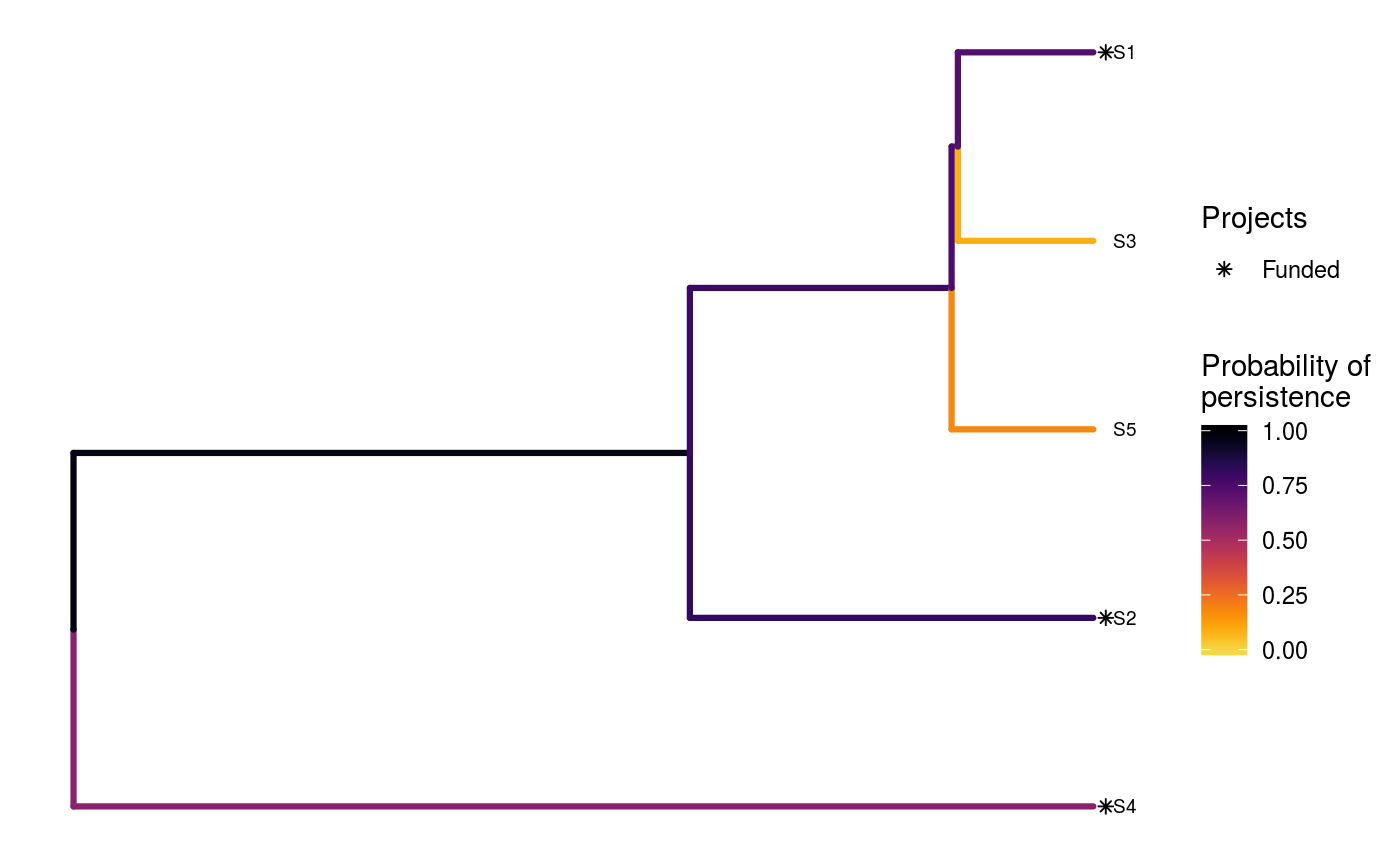
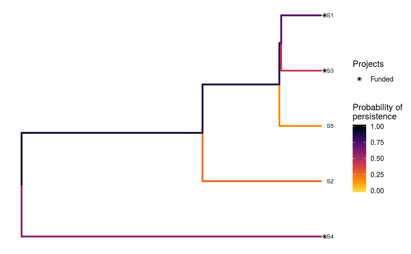
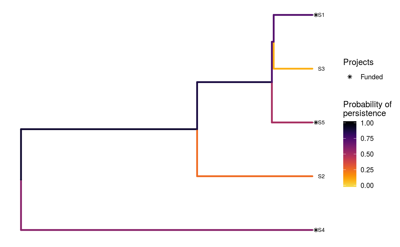
# load built-in data data(sim_project_data, sim_action_data, sim_tree) # print simulated project data set print(sim_project_data)#> # A tibble: 6 x 13 #> name success S1 S2 S3 S4 S5 S1_action S2_action S3_action #> <chr> <dbl> <dbl> <dbl> <dbl> <dbl> <dbl> <lgl> <lgl> <lgl> #> 1 S1_p… 0.919 0.791 0 0 0 0 TRUE FALSE FALSE #> 2 S2_p… 0.923 0 0.888 0 0 0 FALSE TRUE FALSE #> 3 S3_p… 0.829 0 0 0.502 0 0 FALSE FALSE TRUE #> 4 S4_p… 0.848 0 0 0 0.690 0 FALSE FALSE FALSE #> 5 S5_p… 0.814 0 0 0 0 0.617 FALSE FALSE FALSE #> 6 base… 1 0.298 0.250 0.0865 0.249 0.182 FALSE FALSE FALSE #> # ... with 3 more variables: S4_action <lgl>, S5_action <lgl>, #> # baseline_action <lgl>#> # A tibble: 6 x 4 #> name cost locked_in locked_out #> <chr> <dbl> <lgl> <lgl> #> 1 S1_action 94.4 FALSE FALSE #> 2 S2_action 101. FALSE FALSE #> 3 S3_action 103. TRUE FALSE #> 4 S4_action 99.2 FALSE FALSE #> 5 S5_action 99.9 FALSE TRUE #> 6 baseline_action 0 FALSE FALSE#> #> Phylogenetic tree with 5 tips and 4 internal nodes. #> #> Tip labels: #> [1] "S3" "S1" "S5" "S2" "S4" #> #> Rooted; includes branch lengths.# verify if guorbi package is installed if (!require(gurobi, quietly = TRUE)) stop("the gurobi R package is not installed.") # find a solution that meets a budget of 300 s1 <- ppp_exact_phylo_solution(sim_project_data, sim_action_data, sim_tree, 300, "name", "success", "name", "cost") # print solution print(s1)#> # A tibble: 1 x 12 #> solution method obj budget cost optimal S1_action S2_action S3_action #> <int> <chr> <dbl> <dbl> <dbl> <lgl> <lgl> <lgl> <lgl> #> 1 1 exact 2.92 300 295. TRUE TRUE TRUE FALSE #> # ... with 3 more variables: S4_action <lgl>, S5_action <lgl>, #> # baseline_action <lgl># plot solution ppp_plot_phylo_solution(sim_project_data, sim_action_data, sim_tree, s1, "name", "success", "name", "cost")# find a solution that meets a budget of 300 and allocates # funding for the "S3_action" action. For instance, species "S3" might # be an iconic species that has cultural and economic importance. sim_action_data2 <- sim_action_data sim_action_data2$locked_in <- sim_action_data2$name == "S3_action" s2 <- ppp_exact_phylo_solution(sim_project_data, sim_action_data2, sim_tree, 300, "name", "success", "name", "cost", locked_in_column_name = "locked_in") # print solution print(s2)#> # A tibble: 1 x 12 #> solution method obj budget cost optimal S1_action S2_action S3_action #> <int> <chr> <dbl> <dbl> <dbl> <lgl> <lgl> <lgl> <lgl> #> 1 1 exact 2.60 300 297. TRUE TRUE FALSE TRUE #> # ... with 3 more variables: S4_action <lgl>, S5_action <lgl>, #> # baseline_action <lgl># plot solution ppp_plot_phylo_solution(sim_project_data, sim_action_data2, sim_tree, s2, "name", "success", "name", "cost")# find a solution that meets a budget of 300 and does not allocate # funding for the "S2_action" project. For instance, species "S2" # might have very little cultural or economic importance. Broadly speaking, # though, it is better to "lock in" "important" species rather than # "lock out" unimportant species. sim_action_data3 <- sim_action_data sim_action_data3$locked_out <- sim_action_data3$name == "S2_action" s3 <- ppp_exact_phylo_solution(sim_project_data, sim_action_data3, sim_tree, 300, "name", "success", "name", "cost", locked_out_column_name = "locked_out") # print solution print(s3)#> # A tibble: 1 x 12 #> solution method obj budget cost optimal S1_action S2_action S3_action #> <int> <chr> <dbl> <dbl> <dbl> <lgl> <lgl> <lgl> <lgl> #> 1 1 exact 2.61 300 294. TRUE TRUE FALSE FALSE #> # ... with 3 more variables: S4_action <lgl>, S5_action <lgl>, #> # baseline_action <lgl># plot solution ppp_plot_phylo_solution(sim_project_data, sim_action_data3, sim_tree, s3, "name", "success", "name", "cost")# find the top solutions s4 <- ppp_exact_phylo_solution(sim_project_data, sim_action_data, sim_tree, 300, "name", "success", "name", "cost", number_solutions = 1000)#> Warning: although 1000 requested, only 23 solutions exist.#> # A tibble: 23 x 12 #> solution method obj budget cost optimal S1_action S2_action S3_action #> <int> <chr> <dbl> <dbl> <dbl> <lgl> <lgl> <lgl> <lgl> #> 1 1 exact 2.92 300 295. TRUE TRUE TRUE FALSE #> 2 2 exact 2.82 300 295. FALSE TRUE TRUE FALSE #> 3 3 exact 2.64 300 200. FALSE FALSE TRUE FALSE #> 4 4 exact 2.61 300 294. FALSE TRUE FALSE FALSE #> 5 5 exact 2.60 300 297. FALSE TRUE FALSE TRUE #> 6 6 exact 2.50 300 295. FALSE TRUE TRUE FALSE #> 7 7 exact 2.50 300 299. FALSE TRUE TRUE TRUE #> 8 8 exact 2.45 300 194. FALSE TRUE FALSE FALSE #> 9 9 exact 2.39 300 294. FALSE TRUE FALSE FALSE #> 10 10 exact 2.38 300 195. FALSE TRUE TRUE FALSE #> # ... with 13 more rows, and 3 more variables: S4_action <lgl>, #> # S5_action <lgl>, baseline_action <lgl>


