Overview
The optimalppp R package provides methods for prioritizing funding of conservation projects using the ‘Protect Prioritization Protocol’. Projects can be prioritized by maximizing expected species richness or expected phylogenetic diversity. Prioritizations can be generated using a range of methods, such as exact algorithms which can identify optimal solutions, heuristic algorithms which have conventionally been used to identify solutions, and by randomly funding actions. This package also provides the functionality to visualize how well solutions maintain biodiversity.
Tutorial
Here we will provide a short example showing how the optimalppp R package can be used to prioritize funding for conservation projects. With limited resources available for conservation (Balmford et al. 2003), it is imperative that funds are prioritized for conservation projects which will create the best outcome. This realization led to development of the ‘Project Prioritization Protocol’ (Joseph et al. 2009). This protocol, broadly speaking, involves evaluating conservation projects according to (i) the probability that they are expected to succeed, (ii) the probability that species will persist if their projects are funded and successful, and (iii) a metric describing the value of the conserved species (evaluated in Bennett et al. 2014). Since its inception, project prioritization has diverged into ‘species prioritization’ (e.g. Bennett et al. 2014), where each conservation project corresponds to a different species, and ‘priority threat management prioritization’ (Chadés et al. 2015), where each conservation project pertains to a different threat which can affect multiple species. Here we do not differentiate between these types of problems—the optimalppp R package solves a general mathematical formulation that can handle both classes of problems.
The optimalppp R package provides two metrics for prioritizing and evaluating conservation projects. Firstly, prioritizations can be generated by maximizing ‘expected weighted species richness’. This metric is simply the sum of the species’ probabilities of persistence multiplied by their weights (e.g. based on cultural importance or evolutionary significance; e.g. Faith 1992; Gerber et al. 2018). Secondly, prioritizations can be generated by maximizing ‘expected phylogenetic diversity’ (Faith 1992, 2008). This metric uses phylogenetic data to quantify the amount of evolutionary history that is expected to persist into the future. Based on these metrics, prioritizations can be generated under a fixed budget by using exact algorithms (via the Gurobi optimization suite), heuristic algorithms (similar to Bennett et al. 2014), and random processes.
Data simulation
To start off, we will set the seed for the random number generator to ensure reproducibility, load the optimalppp R package, and load the ggtree R package to plot phylogenetic trees. Please note that you will need install the ggtree R package from Bioconductor since it is not available on The Comprehensive R Archive Network (CRAN). This can be achieved with the following command source("https://bioconductor.org/biocLite.R");biocLite("ggtree").
Now we will simulate a data set. This data set will contain conservation projects and conservation actions for 50 species. It will also contain species weight data. And also phylogenetic data that describe the evolutionary relationships between them. To learn more about what these parameters mean, check out ?ppp_simulate_data.
# set simulation parameters
number_species <- 50
cost_mean <- 100
cost_sd <- 5
success_min_probability <- 0.7
success_max_probability <- 0.99
funded_min_persistence_probability <- 0.5
funded_max_persistence_probability <- 0.9
not_funded_min_persistence_probability <- 0.01
not_funded_max_persistence_probability <- 0.4
locked_in_proportion <- 0.1
locked_out_proportion <- 0.1

# simulate data
sim <- ppp_simulate_data(number_species,
                         cost_mean,
                         cost_sd,
                         success_min_probability,
                         success_max_probability,
                         funded_min_persistence_probability,
                         funded_max_persistence_probability,
                         not_funded_min_persistence_probability,
                         not_funded_max_persistence_probability,
                         locked_in_proportion,
                         locked_out_proportion)

# extract the data
project_data <- sim$project_data
action_data <- sim$action_data
species_data <- sim$species_data
tree <- sim$tree
Now let’s examine the simulated data. Let’s look at the action_data object. This object stores information about various conservation actions in a tabular format (i.e. tibble). Each row corresponds to a different action, and each column describes different properties associated with the actions. These actions correspond to specific management actions that have known costs. For example, they may relate to baiting or trapping sites of conservation importance. In this table, the "name" column contains the name of each action, and the "cost" action denotes the cost of funding each project. It also contains additional columns for customizing the solutions, but we will ignore them for now. Note that the last project—the "baseline_action"—has a zero cost and is used subsequently to represent the baseline probability for species when no conservation actions are funded for them.
# preview first six rows of the table
head(as.data.frame(action_data))
## name cost locked_in locked_out
## 1 S1_action 99.56090 FALSE FALSE
## 2 S2_action 98.85517 FALSE TRUE
## 3 S3_action 99.57851 FALSE FALSE
## 4 S4_action 91.29526 TRUE FALSE
## 5 S5_action 105.06716 FALSE FALSE
## 6 S6_action 98.91054 FALSE FALSENext, let’s examine the project_data object. This object stores information about various conservation projects in a tabular format (i.e. tibble). Each row corresponds to a different project, and each column describes various properties associated with the projects. Each project is associated with a single or multiple conservation actions (in the action_data object). For example, a conservation project may pertain to a set of conservation actions that relate to a single species or single geographic locality. In this table, the "name" column contains the name of each project, the "success" column denotes the probability of each project succeeding if it is funded, the "S1"–"SN" columns show the enhanced probability of each species persisting if the project is funded (where zeros mean that a species does not benefit from a project), and the "S1_action"–"SN_action" columns indicate which actions are associated with which projects. Note that the last project—the "baseline_project"—is associated with the "baseline_action" action. This project has a zero cost and represents the baseline probability of each species persisting if no other project is funded. Finally, although most projects in this example directly relate to a single species, you can input projects that directly affect the persistence of multiple species—you simply need to adjust the species persistence probabilities in the table. This format means that the optimalppp R package can be used to solve problems that are classically considered ‘species prioritization’ or ‘priority threat management’ problems.
# preview first six rows of the table
head(as.data.frame(project_data))
## name success S1 S10 S11 S12 S13
## 1 S1_project 0.8616642 0.6199881 0.0000000 0.0000000 0.0000000 0.0000000
## 2 S2_project 0.8160988 0.0000000 0.6209851 0.0000000 0.0000000 0.0000000
## 3 S3_project 0.7018839 0.0000000 0.0000000 0.7495242 0.0000000 0.0000000
## 4 S4_project 0.7427809 0.0000000 0.0000000 0.0000000 0.5287815 0.0000000
## 5 S5_project 0.8139378 0.0000000 0.0000000 0.0000000 0.0000000 0.6540845
## 6 S6_project 0.9800510 0.0000000 0.0000000 0.0000000 0.0000000 0.0000000
## S14 S15 S16 S17 S18 S19 S2 S20 S21 S22 S23 S24 S25 S26 S27 S28 S29
## 1 0.0000000 0 0 0 0 0 0 0 0 0 0 0 0 0 0 0 0
## 2 0.0000000 0 0 0 0 0 0 0 0 0 0 0 0 0 0 0 0
## 3 0.0000000 0 0 0 0 0 0 0 0 0 0 0 0 0 0 0 0
## 4 0.0000000 0 0 0 0 0 0 0 0 0 0 0 0 0 0 0 0
## 5 0.0000000 0 0 0 0 0 0 0 0 0 0 0 0 0 0 0 0
## 6 0.7916949 0 0 0 0 0 0 0 0 0 0 0 0 0 0 0 0
## S3 S30 S31 S32 S33 S34 S35 S36 S37 S38 S39 S4 S40 S41 S42 S43 S44 S45
## 1 0 0 0 0 0 0 0 0 0 0 0 0 0 0 0 0 0 0
## 2 0 0 0 0 0 0 0 0 0 0 0 0 0 0 0 0 0 0
## 3 0 0 0 0 0 0 0 0 0 0 0 0 0 0 0 0 0 0
## 4 0 0 0 0 0 0 0 0 0 0 0 0 0 0 0 0 0 0
## 5 0 0 0 0 0 0 0 0 0 0 0 0 0 0 0 0 0 0
## 6 0 0 0 0 0 0 0 0 0 0 0 0 0 0 0 0 0 0
## S46 S47 S48 S49 S5 S50 S6 S7 S8 S9 S1_action S2_action S3_action
## 1 0 0 0 0 0 0 0 0 0 0 TRUE FALSE FALSE
## 2 0 0 0 0 0 0 0 0 0 0 FALSE TRUE FALSE
## 3 0 0 0 0 0 0 0 0 0 0 FALSE FALSE TRUE
## 4 0 0 0 0 0 0 0 0 0 0 FALSE FALSE FALSE
## 5 0 0 0 0 0 0 0 0 0 0 FALSE FALSE FALSE
## 6 0 0 0 0 0 0 0 0 0 0 FALSE FALSE FALSE
## S4_action S5_action S6_action S7_action S8_action S9_action S10_action
## 1 FALSE FALSE FALSE FALSE FALSE FALSE FALSE
## 2 FALSE FALSE FALSE FALSE FALSE FALSE FALSE
## 3 FALSE FALSE FALSE FALSE FALSE FALSE FALSE
## 4 TRUE FALSE FALSE FALSE FALSE FALSE FALSE
## 5 FALSE TRUE FALSE FALSE FALSE FALSE FALSE
## 6 FALSE FALSE TRUE FALSE FALSE FALSE FALSE
## S11_action S12_action S13_action S14_action S15_action S16_action
## 1 FALSE FALSE FALSE FALSE FALSE FALSE
## 2 FALSE FALSE FALSE FALSE FALSE FALSE
## 3 FALSE FALSE FALSE FALSE FALSE FALSE
## 4 FALSE FALSE FALSE FALSE FALSE FALSE
## 5 FALSE FALSE FALSE FALSE FALSE FALSE
## 6 FALSE FALSE FALSE FALSE FALSE FALSE
## S17_action S18_action S19_action S20_action S21_action S22_action
## 1 FALSE FALSE FALSE FALSE FALSE FALSE
## 2 FALSE FALSE FALSE FALSE FALSE FALSE
## 3 FALSE FALSE FALSE FALSE FALSE FALSE
## 4 FALSE FALSE FALSE FALSE FALSE FALSE
## 5 FALSE FALSE FALSE FALSE FALSE FALSE
## 6 FALSE FALSE FALSE FALSE FALSE FALSE
## S23_action S24_action S25_action S26_action S27_action S28_action
## 1 FALSE FALSE FALSE FALSE FALSE FALSE
## 2 FALSE FALSE FALSE FALSE FALSE FALSE
## 3 FALSE FALSE FALSE FALSE FALSE FALSE
## 4 FALSE FALSE FALSE FALSE FALSE FALSE
## 5 FALSE FALSE FALSE FALSE FALSE FALSE
## 6 FALSE FALSE FALSE FALSE FALSE FALSE
## S29_action S30_action S31_action S32_action S33_action S34_action
## 1 FALSE FALSE FALSE FALSE FALSE FALSE
## 2 FALSE FALSE FALSE FALSE FALSE FALSE
## 3 FALSE FALSE FALSE FALSE FALSE FALSE
## 4 FALSE FALSE FALSE FALSE FALSE FALSE
## 5 FALSE FALSE FALSE FALSE FALSE FALSE
## 6 FALSE FALSE FALSE FALSE FALSE FALSE
## S35_action S36_action S37_action S38_action S39_action S40_action
## 1 FALSE FALSE FALSE FALSE FALSE FALSE
## 2 FALSE FALSE FALSE FALSE FALSE FALSE
## 3 FALSE FALSE FALSE FALSE FALSE FALSE
## 4 FALSE FALSE FALSE FALSE FALSE FALSE
## 5 FALSE FALSE FALSE FALSE FALSE FALSE
## 6 FALSE FALSE FALSE FALSE FALSE FALSE
## S41_action S42_action S43_action S44_action S45_action S46_action
## 1 FALSE FALSE FALSE FALSE FALSE FALSE
## 2 FALSE FALSE FALSE FALSE FALSE FALSE
## 3 FALSE FALSE FALSE FALSE FALSE FALSE
## 4 FALSE FALSE FALSE FALSE FALSE FALSE
## 5 FALSE FALSE FALSE FALSE FALSE FALSE
## 6 FALSE FALSE FALSE FALSE FALSE FALSE
## S47_action S48_action S49_action S50_action baseline_action
## 1 FALSE FALSE FALSE FALSE FALSE
## 2 FALSE FALSE FALSE FALSE FALSE
## 3 FALSE FALSE FALSE FALSE FALSE
## 4 FALSE FALSE FALSE FALSE FALSE
## 5 FALSE FALSE FALSE FALSE FALSE
## 6 FALSE FALSE FALSE FALSE FALSENext up, let’s look at the species_data object. This object stores information about each species in tabular format. Here, each row corresponds to a different species and each column contains information about the species. It contains a "name" column which denotes the name of each species. Note that these names also appear as column names in the project_data object. It also contains a "weight" column that denotes the relative importance of each species. These weights reflect the evolutionary significance of each species, though they could also reflect cultural or economic importance too. You would simply need to adjust the values accordingly.
# preview first six rows of the table
head(as.data.frame(species_data))
## name weight
## 1 S25 0.0395923212
## 2 S9 0.0002666836
## 3 S11 0.0002666836
## 4 S12 0.0771402026
## 5 S34 0.0691797469
## 6 S6 0.0318333994Finally, let’s look at the tree object. This object stores information about the evolutionary relationships between the simulated species. If you want to read in your own phylogenetic data, check out the read.nexus function from the ape R package. Using this object, we can make a plot—specifically, a phylogram—depicting the evolutionary history of our simulated species.
# plot tree
ggtree(tree) +
geom_tiplab(size = 2.5)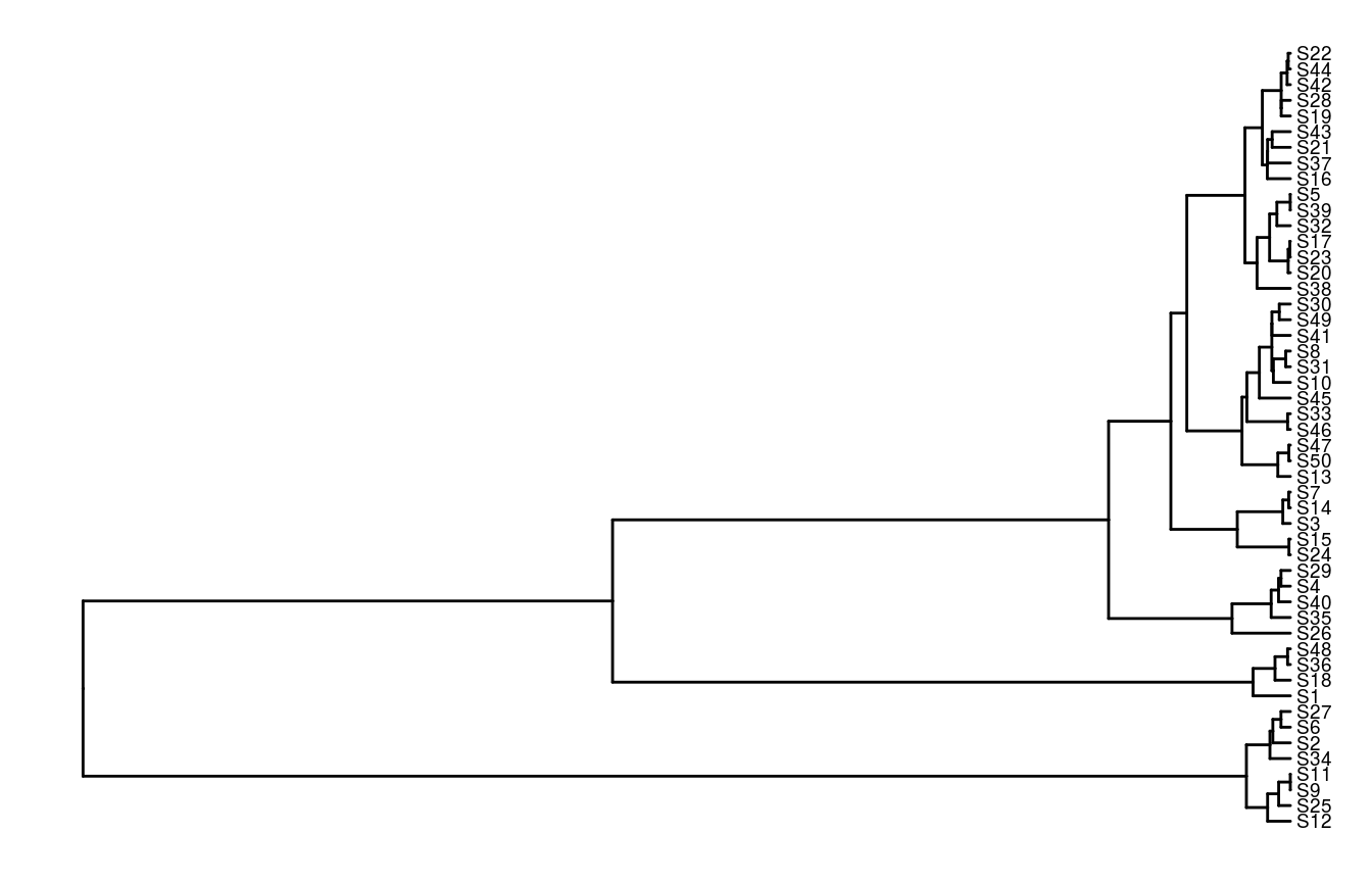
Maximizing expected weighted species richness
Now let’s generate some prioritizations using the simulated data. Specifically, we will generate prioritizations using the ‘expected weighted species richness’ metric. This metric is calculated by multiplying the probability that each species is expected to persist by the species’ weight value and summing these values together. It is often used in situations where phylogenetic data are not available. Let us assume that our resources are limited such that we can only spend, at most, $500 on funding conservation projects. In other words, our budget is capped at $500. Now, given the project data (project_data), the action data (action_data), the species data (species_data), and this budget (500), we can begin prioritizing funding for the conservation projects. Conventionally, conservation projects have been prioritized using heuristic algorithms (e.g. Bennett et al. 2014), so let’s generate our first prioritization using these algorithms.
# prioritize funding using heuristic algorithm
s1 <- ppp_heuristic_spp_solution(x = project_data, y = action_data,
                                 spp =  species_data, budget = 500,
                                 project_column_name = "name",
                                 success_column_name = "success",
                                 action_column_name = "name",
                                 cost_column_name = "cost",
                                 species_column_name = "name",
                                 weight_column_name = "weight")

# print solution
print(s1)
## # A tibble: 1 x 57
## solution method obj budget cost optimal S1_action S2_action S3_action
## <int> <chr> <dbl> <dbl> <dbl> <lgl> <lgl> <lgl> <lgl>
## 1 1 heuri… 0.591 500 409. NA FALSE FALSE FALSE
## # ... with 48 more variables: S4_action <lgl>, S5_action <lgl>,
## # S6_action <lgl>, S7_action <lgl>, S8_action <lgl>, S9_action <lgl>,
## # S10_action <lgl>, S11_action <lgl>, S12_action <lgl>,
## # S13_action <lgl>, S14_action <lgl>, S15_action <lgl>,
## # S16_action <lgl>, S17_action <lgl>, S18_action <lgl>,
## # S19_action <lgl>, S20_action <lgl>, S21_action <lgl>,
## # S22_action <lgl>, S23_action <lgl>, S24_action <lgl>,
## # S25_action <lgl>, S26_action <lgl>, S27_action <lgl>,
## # S28_action <lgl>, S29_action <lgl>, S30_action <lgl>,
## # S31_action <lgl>, S32_action <lgl>, S33_action <lgl>,
## # S34_action <lgl>, S35_action <lgl>, S36_action <lgl>,
## # S37_action <lgl>, S38_action <lgl>, S39_action <lgl>,
## # S40_action <lgl>, S41_action <lgl>, S42_action <lgl>,
## # S43_action <lgl>, S44_action <lgl>, S45_action <lgl>,
## # S46_action <lgl>, S47_action <lgl>, S48_action <lgl>,
## # S49_action <lgl>, S50_action <lgl>, baseline_action <lgl>The object s1 contains the solution and also various statistics associated with the solution in a tabular format (i.e. tibble). Here, each row corresponds to a different solution. Specifically, the "solution" column contains an identifier for each solution (this is useful for methods that output multiple solutions), the "obj" column contains the objective value (i.e. the expected weighted species richness), the "budget" column stores the budget used for generating the solution, the "cost" column stores the cost of the solution, the "optimal" column indicates if the solution is known to be optimal (NA values mean the optimality is unknown), and the "method" column contains the name of the method used to generate the solution. The remaining columns ("S1_project", "S2_project", "S3_project", …, "S50_project", and "baseline_project") indicate if a given project was prioritized for funding (TRUE) or not (FALSE).
To help interpret this solution, let’s make a plot. In this plot, each line corresponds to a different species. The length of each line represents the species’ weight, and the color of each line indicates the probability that each species is expected to persist. Asterisk symbols indicate which species benefit from funded projects which have all of their actions funded.
# visualize solution
ppp_plot_spp_solution(project_data, action_data, species_data, s1,
                      project_column_name = "name",
                      success_column_name = "success",
                      action_column_name = "name",
                      cost_column_name = "cost",
                      species_column_name = "name",
                      weight_column_name = "weight",
                      symbol_hjust = 0.01)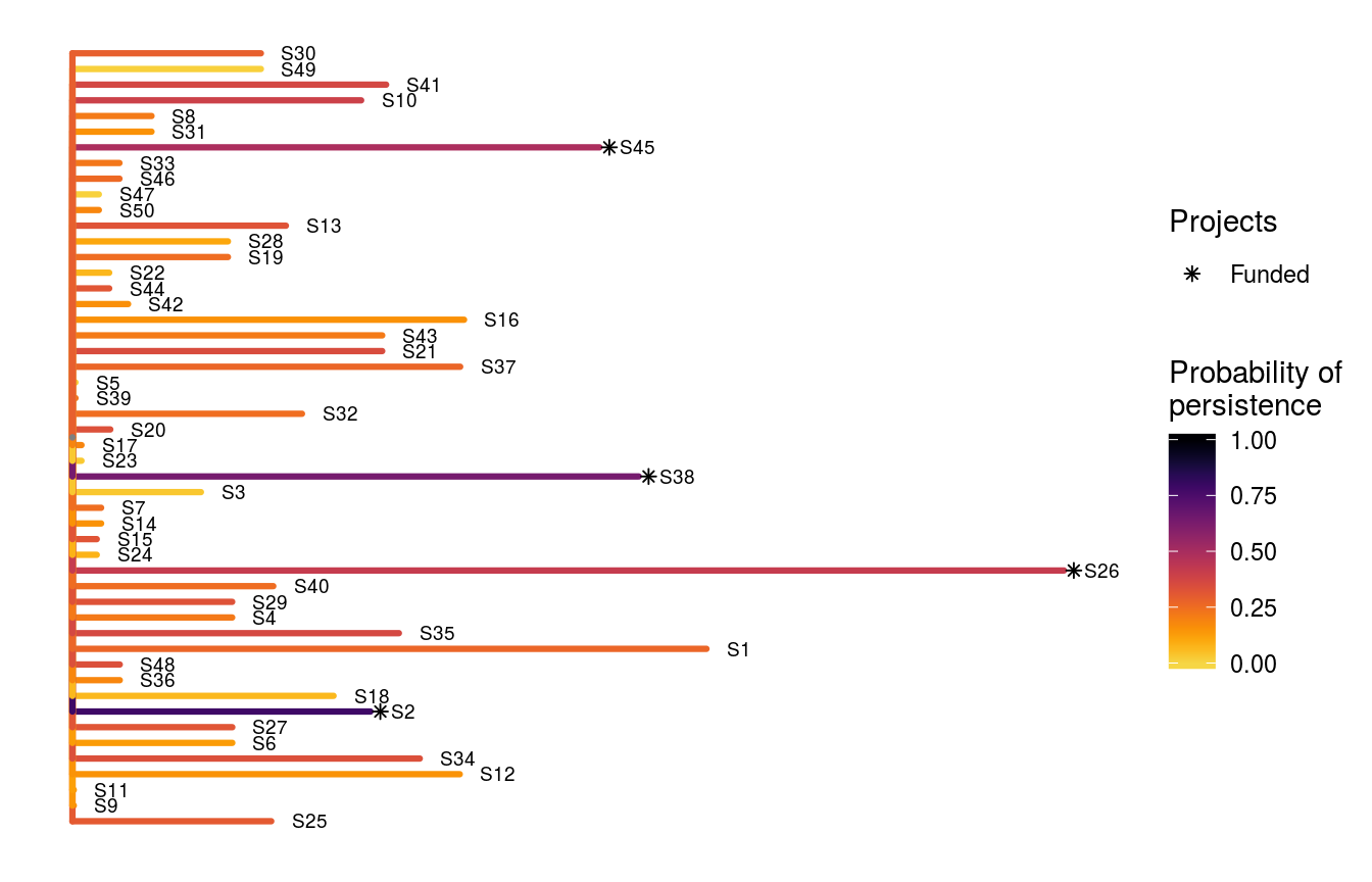
In some cases, we might have projects for iconic species that are socially and economically important. To ensure that actions for these species are funded—regardless of cost-efficiency or benefit—we can “lock in” certain projects into the solution (conversely, we can also “lock out” certain actions if desired too). Although we could simply increase the weighting for such species, “locking in” such species provides a more transparent approach. Let us imagine that it is absolutely critical that the action for species S1 (named "S1_action") receives funding. Let’s generate a solution using the heuristic algorithm with this constraint.
# set locked in column to only lock in species S1
action_data$locked_in <- action_data$name == "S1_action"

# prioritize funding using heuristic algorithm
s2 <- ppp_heuristic_spp_solution(x = project_data, y = action_data,
                                 spp = species_data, budget = 500,
                                 project_column_name = "name",
                                 success_column_name = "success",
                                 action_column_name = "name",
                                 cost_column_name = "cost",
                                 species_column_name = "name",
                                 weight_column_name = "weight",
                                 locked_in_column_name = "locked_in")

# print solution
print(s2)
## # A tibble: 1 x 57
## solution method obj budget cost optimal S1_action S2_action S3_action
## <int> <chr> <dbl> <dbl> <dbl> <lgl> <lgl> <lgl> <lgl>
## 1 1 heuri… 0.585 500 407. NA TRUE FALSE FALSE
## # ... with 48 more variables: S4_action <lgl>, S5_action <lgl>,
## # S6_action <lgl>, S7_action <lgl>, S8_action <lgl>, S9_action <lgl>,
## # S10_action <lgl>, S11_action <lgl>, S12_action <lgl>,
## # S13_action <lgl>, S14_action <lgl>, S15_action <lgl>,
## # S16_action <lgl>, S17_action <lgl>, S18_action <lgl>,
## # S19_action <lgl>, S20_action <lgl>, S21_action <lgl>,
## # S22_action <lgl>, S23_action <lgl>, S24_action <lgl>,
## # S25_action <lgl>, S26_action <lgl>, S27_action <lgl>,
## # S28_action <lgl>, S29_action <lgl>, S30_action <lgl>,
## # S31_action <lgl>, S32_action <lgl>, S33_action <lgl>,
## # S34_action <lgl>, S35_action <lgl>, S36_action <lgl>,
## # S37_action <lgl>, S38_action <lgl>, S39_action <lgl>,
## # S40_action <lgl>, S41_action <lgl>, S42_action <lgl>,
## # S43_action <lgl>, S44_action <lgl>, S45_action <lgl>,
## # S46_action <lgl>, S47_action <lgl>, S48_action <lgl>,
## # S49_action <lgl>, S50_action <lgl>, baseline_action <lgl>Let’s visualize this new solution with species S1 locked in.
# visualize solution
ppp_plot_spp_solution(project_data, action_data, species_data, s2,
                      project_column_name = "name",
                      success_column_name = "success",
                      action_column_name = "name",
                      cost_column_name = "cost",
                      species_column_name = "name",
                      weight_column_name = "weight",
                      symbol_hjust = 0.01)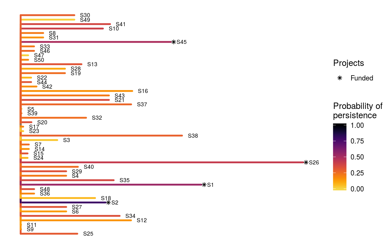
Next, we might want to evaluate how well this solution compares to funding conservation actions at random. To achieve this, we need to generate solutions that contain randomly selected actions that (i) always include the baseline scenario project, and (ii) meet the budget. Fortunately, the ppp_random_spp_solution function does this for us. So, let’s generate 1,000 random solutions with a budget of $500.
# prioritize funding using random processes
s3 <- ppp_random_spp_solution(x = project_data, y = action_data,
                              spp = species_data, budget = 500,
                              project_column_name = "name",
                              success_column_name = "success",
                              action_column_name = "name",
                              cost_column_name = "cost",
                              species_column_name = "name",
                              weight_column_name = "weight",
                              locked_in_column_name = "locked_in",
                              number_solutions = 1000)

# print solution
print(s3)
## # A tibble: 1,000 x 57
## solution method obj budget cost optimal S1_action S2_action S3_action
## <int> <chr> <dbl> <dbl> <dbl> <lgl> <lgl> <lgl> <lgl>
## 1 1 random 0.497 500 408. NA TRUE FALSE FALSE
## 2 2 random 0.485 500 489. NA TRUE FALSE FALSE
## 3 3 random 0.461 500 414. NA TRUE FALSE FALSE
## 4 4 random 0.442 500 401. NA TRUE FALSE FALSE
## 5 5 random 0.501 500 491. NA TRUE FALSE FALSE
## 6 6 random 0.551 500 499. NA TRUE FALSE FALSE
## 7 7 random 0.457 500 494. NA TRUE FALSE FALSE
## 8 8 random 0.450 500 497. NA TRUE FALSE FALSE
## 9 9 random 0.453 500 497. NA TRUE TRUE FALSE
## 10 10 random 0.439 500 401. NA TRUE FALSE FALSE
## # ... with 990 more rows, and 48 more variables: S4_action <lgl>,
## # S5_action <lgl>, S6_action <lgl>, S7_action <lgl>, S8_action <lgl>,
## # S9_action <lgl>, S10_action <lgl>, S11_action <lgl>, S12_action <lgl>,
## # S13_action <lgl>, S14_action <lgl>, S15_action <lgl>,
## # S16_action <lgl>, S17_action <lgl>, S18_action <lgl>,
## # S19_action <lgl>, S20_action <lgl>, S21_action <lgl>,
## # S22_action <lgl>, S23_action <lgl>, S24_action <lgl>,
## # S25_action <lgl>, S26_action <lgl>, S27_action <lgl>,
## # S28_action <lgl>, S29_action <lgl>, S30_action <lgl>,
## # S31_action <lgl>, S32_action <lgl>, S33_action <lgl>,
## # S34_action <lgl>, S35_action <lgl>, S36_action <lgl>,
## # S37_action <lgl>, S38_action <lgl>, S39_action <lgl>,
## # S40_action <lgl>, S41_action <lgl>, S42_action <lgl>,
## # S43_action <lgl>, S44_action <lgl>, S45_action <lgl>,
## # S46_action <lgl>, S47_action <lgl>, S48_action <lgl>,
## # S49_action <lgl>, S50_action <lgl>, baseline_action <lgl>Let’s visualize the first solution in the set of 1,000 randomly generated solutions.
# visualize solution
ppp_plot_spp_solution(project_data, action_data, species_data, s3,
                      project_column_name = "name",
                      success_column_name = "success",
                      action_column_name = "name",
                      cost_column_name = "cost",
                      species_column_name = "name",
                      weight_column_name = "weight",
                      symbol_hjust = 0.01, n = 1)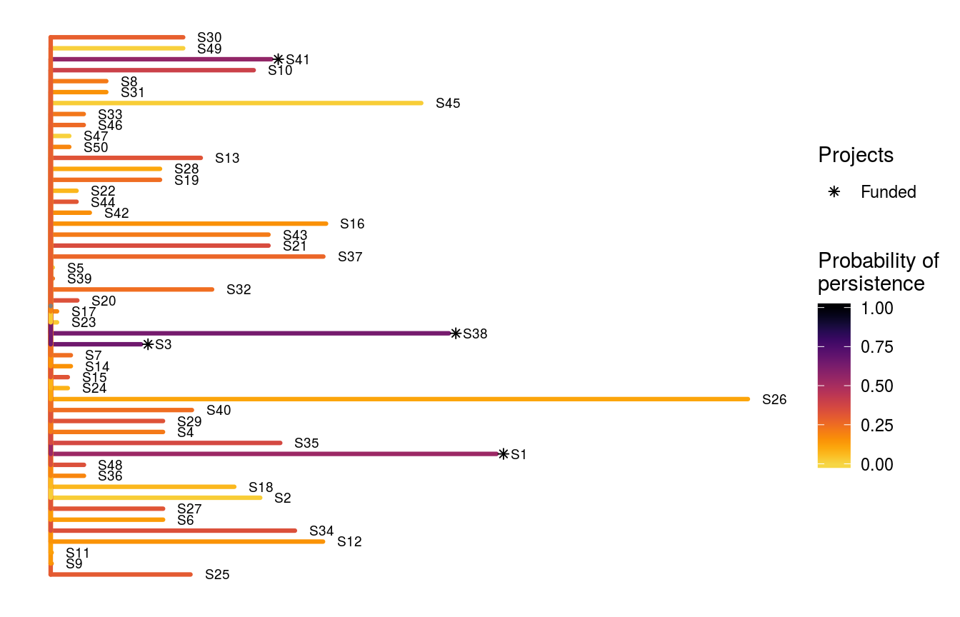
We can now calculate how much better the solution generated using the heuristic algorithm performs than randomly funding conservation actions.
## [1] 0.2336022Since the heuristic algorithm performs better than random, you might be tempted to think that the heuristic algorithm is pretty good. But you would be wrong. This is because the heuristic algorithms provide no guarantees on solution quality relative to optimality. This is because objective value associated with a solution tells us how good the solution is, but it does not tell us how good the solution is compared to the best possible solution (i.e. optimality). Therefore we cannot possibly be confident that the solution is any good at all. Fortunately, we can use exact algorithms to find the optimal solution to this problem (for discussion on exact algorithms in conservation, see Underhill 1994; Rodrigues & Gaston 2002).
# prioritize funding using exact algorithm
s4 <- ppp_exact_spp_solution(x = project_data, y = action_data,
                             spp = species_data, budget = 500,
                             project_column_name = "name",
                             success_column_name = "success",
                             action_column_name = "name",
                             cost_column_name = "cost",
                             species_column_name = "name",
                             weight_column_name = "weight",
                             locked_in_column_name = "locked_in")

# print solution
print(s4)
## # A tibble: 1 x 57
## solution method obj budget cost optimal S1_action S2_action S3_action
## <int> <chr> <dbl> <dbl> <dbl> <lgl> <lgl> <lgl> <lgl>
## 1 1 exact 0.603 500 498. TRUE TRUE FALSE FALSE
## # ... with 48 more variables: S4_action <lgl>, S5_action <lgl>,
## # S6_action <lgl>, S7_action <lgl>, S8_action <lgl>, S9_action <lgl>,
## # S10_action <lgl>, S11_action <lgl>, S12_action <lgl>,
## # S13_action <lgl>, S14_action <lgl>, S15_action <lgl>,
## # S16_action <lgl>, S17_action <lgl>, S18_action <lgl>,
## # S19_action <lgl>, S20_action <lgl>, S21_action <lgl>,
## # S22_action <lgl>, S23_action <lgl>, S24_action <lgl>,
## # S25_action <lgl>, S26_action <lgl>, S27_action <lgl>,
## # S28_action <lgl>, S29_action <lgl>, S30_action <lgl>,
## # S31_action <lgl>, S32_action <lgl>, S33_action <lgl>,
## # S34_action <lgl>, S35_action <lgl>, S36_action <lgl>,
## # S37_action <lgl>, S38_action <lgl>, S39_action <lgl>,
## # S40_action <lgl>, S41_action <lgl>, S42_action <lgl>,
## # S43_action <lgl>, S44_action <lgl>, S45_action <lgl>,
## # S46_action <lgl>, S47_action <lgl>, S48_action <lgl>,
## # S49_action <lgl>, S50_action <lgl>, baseline_action <lgl>Now let’s visualize the optimal solution.
# visualize solution
ppp_plot_spp_solution(project_data, action_data, species_data, s4,
                      project_column_name = "name",
                      success_column_name = "success",
                      action_column_name = "name",
                      cost_column_name = "cost",
                      species_column_name = "name",
                      weight_column_name = "weight",
                      symbol_hjust = 0.01)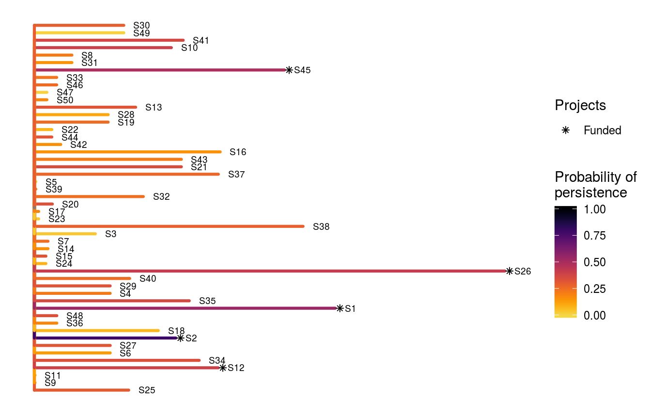
Now that we have the optimal solution (objective value = 0.603), we can see that the solution generated by the heuristic algorithm (objective value = 0.585) was indeed suboptimal.
Expected phylogenetic diversity
Now that we’ve tried prioritizing projects using the species weights, let’s try using the phylogentic data. We can achieve this using the tree object instead of the species_data object.
# prioritize funding using exact algorithm
s5 <- ppp_exact_phylo_solution(x = project_data, y = action_data,
                               tree = tree, budget = 500,
                               project_column_name = "name",
                               success_column_name = "success",
                               action_column_name = "name",
                               cost_column_name = "cost",
                               locked_in_column_name = "locked_in")

# print solution
print(s5)
## # A tibble: 1 x 57
## solution method obj budget cost optimal S1_action S2_action S3_action
## <int> <chr> <dbl> <dbl> <dbl> <lgl> <lgl> <lgl> <lgl>
## 1 1 exact 12.0 500 485. TRUE TRUE FALSE FALSE
## # ... with 48 more variables: S4_action <lgl>, S5_action <lgl>,
## # S6_action <lgl>, S7_action <lgl>, S8_action <lgl>, S9_action <lgl>,
## # S10_action <lgl>, S11_action <lgl>, S12_action <lgl>,
## # S13_action <lgl>, S14_action <lgl>, S15_action <lgl>,
## # S16_action <lgl>, S17_action <lgl>, S18_action <lgl>,
## # S19_action <lgl>, S20_action <lgl>, S21_action <lgl>,
## # S22_action <lgl>, S23_action <lgl>, S24_action <lgl>,
## # S25_action <lgl>, S26_action <lgl>, S27_action <lgl>,
## # S28_action <lgl>, S29_action <lgl>, S30_action <lgl>,
## # S31_action <lgl>, S32_action <lgl>, S33_action <lgl>,
## # S34_action <lgl>, S35_action <lgl>, S36_action <lgl>,
## # S37_action <lgl>, S38_action <lgl>, S39_action <lgl>,
## # S40_action <lgl>, S41_action <lgl>, S42_action <lgl>,
## # S43_action <lgl>, S44_action <lgl>, S45_action <lgl>,
## # S46_action <lgl>, S47_action <lgl>, S48_action <lgl>,
## # S49_action <lgl>, S50_action <lgl>, baseline_action <lgl>Now let’s visualize this optimal solution based on using phylogenetic data.
# visualize solution
ppp_plot_phylo_solution(project_data, action_data, tree, s5,
                        project_column_name = "name",
                        success_column_name = "success",
                        action_column_name = "name",
                        cost_column_name = "cost",
                        symbol_hjust = 0.01)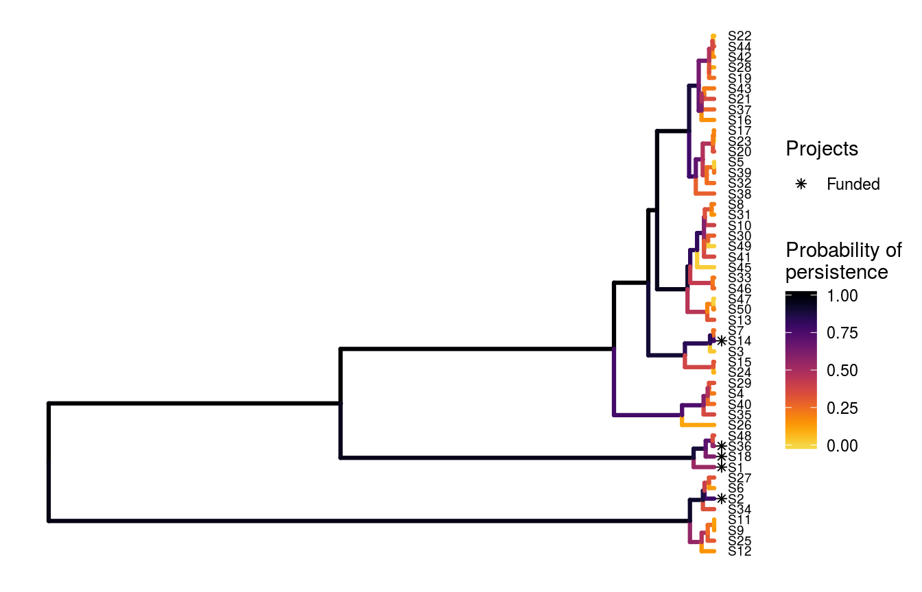
Earlier, we generated a solution using species weights that reflected evolutionary importance (i.e. the s4 object). Let’s compare the optimal solution based on phylogenetic data to the optimal solution based on species weights. To do this, we will use the solution in the s4 object to manually specify a solution for the expected phylogenetic diversity problem.
# evaluate solution based on species weights
s6 <- ppp_manual_phylo_solution(x = project_data, y = action_data, tree = tree,
                                solution = s4[, action_data$name],
                                project_column_name = "name",
                                success_column_name = "success",
                                action_column_name = "name",
                                cost_column_name = "cost")

# print solution
print(s6)
## # A tibble: 1 x 57
## solution method obj budget cost optimal S1_action S2_action S3_action
## <int> <chr> <dbl> <dbl> <dbl> <lgl> <lgl> <lgl> <lgl>
## 1 1 manual 11.6 NA 498. NA TRUE FALSE FALSE
## # ... with 48 more variables: S4_action <lgl>, S5_action <lgl>,
## # S6_action <lgl>, S7_action <lgl>, S8_action <lgl>, S9_action <lgl>,
## # S10_action <lgl>, S11_action <lgl>, S12_action <lgl>,
## # S13_action <lgl>, S14_action <lgl>, S15_action <lgl>,
## # S16_action <lgl>, S17_action <lgl>, S18_action <lgl>,
## # S19_action <lgl>, S20_action <lgl>, S21_action <lgl>,
## # S22_action <lgl>, S23_action <lgl>, S24_action <lgl>,
## # S25_action <lgl>, S26_action <lgl>, S27_action <lgl>,
## # S28_action <lgl>, S29_action <lgl>, S30_action <lgl>,
## # S31_action <lgl>, S32_action <lgl>, S33_action <lgl>,
## # S34_action <lgl>, S35_action <lgl>, S36_action <lgl>,
## # S37_action <lgl>, S38_action <lgl>, S39_action <lgl>,
## # S40_action <lgl>, S41_action <lgl>, S42_action <lgl>,
## # S43_action <lgl>, S44_action <lgl>, S45_action <lgl>,
## # S46_action <lgl>, S47_action <lgl>, S48_action <lgl>,
## # S49_action <lgl>, S50_action <lgl>, baseline_action <lgl>We can see that the solution generated using species weights to account for evolutionary importance (objective value = 11.647) performed worse than the solution generated using phylogenetic data (objective value = 12.042) when evaluated using the phylogenetic data. This result is important because it suggests that conservation prioritizations may benefit by using better quality data.
Finally, let’s examine the trade-off between conservation expenditure and the amount of evolutionary history that is expected to persist. We can achieve this by creating a series of prioritizations using increasing budgets, and then plotting the objective values against the cost of the prioritizations. Here we will use fifty different budgets to reduce run time, though in practice you would use a much larger number (e.g. 10,000) to create a more accurate trade-off curve.
# create a vector of 50 different budgets
budgets <- seq(0, sum(action_data$cost), length.out = 50)

# create prioritizations using different budgets
solution_data <- do.call(rbind, lapply(budgets, ppp_exact_phylo_solution,
                                       x = project_data, y = action_data,
                                       tree = tree,
                                       project_column_name = "name",
                                       success_column_name = "success",
                                       action_column_name = "name",
                                       cost_column_name = "cost"))

# create a data.frame to plot the results
plot_data <- data.frame(cost = seq(0, sum(action_data$cost), length.out = 1e+4))
plot_data$obj <- approx(x = solution_data$cost, y = solution_data$obj,
                        xout = plot_data$cost, method = "constant")$y

# plot relationship between cost and conservation value
plot(obj ~ cost, data = plot_data, type = "l", xlab = "Cost ($)",
     ylab = "Expected phylogenetic diversity (million years)")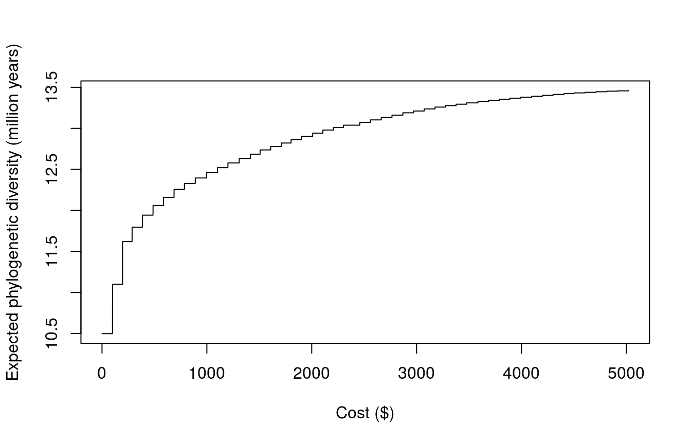
Citation
Please use the following citation to cite the optimalppp R package in publications:
Hanson JO, Schuster R, Strimas-Mackey M, Bennett J, (2018). optimalppp: Optimal Project Prioritization Protocol. R package version 0.0.0.4. Available at https://github.com/prioritizr/optimalppp.
References
Balmford, A., Gaston, K.J., Blyth, S., James, A. & Kapos, V. (2003). Global variation in terrestrial conservation costs, conservation benefits, and unmet conservation needs. Proceedings of the National Academy of Sciences, 100, 1046–1050.
Bennett, J.R., Elliott, G., Mellish, B., Joseph, L.N., Tulloch, A.I., Probert, W.J., Di Fonzo, M.M., Monks, J.M., Possingham, H.P. & Maloney, R. (2014). Balancing phylogenetic diversity and species numbers in conservation prioritizat, using a case study of threatened species in New Zealand. Biological Conservation, 174, 47–54.
Chadés, I., Nicol, S., Leeuwen, S. van, Walters, B., Firn, J., Reeson, A., Martin, T.G. & Carwardine, J. (2015). Benefits of integrating complementarity into priority threat management. Conservation Biology, 29, 525–536.
Faith, D.P. (1992). Conservation evaluation and phylogenetic diversity. Biological Conservation, 61, 1–10.
Faith, D.P. (2008). Threatened species and the potential loss of phylogenetic diversity: Conservation scenarios based on estimated extinction probabilities and phylogenetic risk analysis. Conservation Biology, 22, 1461–1470.
Gerber, L.R., Runge, M.C., Maloney, R.F., Iacona, G.D., Drew, C.A., Avery-Gomm, S., Brazill-Boast, J., Crouse, D., Epanchin-Niell, R.S., Hall, S.B. & others. (2018). Endangered species recovery: A resource allocation problem. Science, 362, 284–286.
Joseph, L.N., Maloney, R.F. & Possingham, H.P. (2009). Optimal allocation of resources among threatened species: A project prioritization protocol. Conservation Biology, 23, 328–338.
Rodrigues, A.S. & Gaston, K.J. (2002). Optimisation in reserve selection procedures—why not? Biological Conservation, 107, 123–129.
Underhill, L. (1994). Optimal and suboptimal reserve selection algorithms. Biological Conservation, 70, 85–87.