Calculate the replacement cost for priority actions in a project
prioritization problem() (Moilanen et al. 2009). Actions associated
with larger replacement cost values are more irreplaceable, and may
need to be implemented sooner than actions with lower replacement cost
values.
replacement_costs(x, solution, n = 1)Arguments
- x
project prioritization
problem().- solution
base::data.frame()ortibble::tibble()table containing the solutions. Here, rows correspond to different solutions and columns correspond to different actions. Each column in the argument tosolutionshould be named according to a different action inx. Cell values indicate if an action is funded in a given solution or not, and should be either zero or one. Arguments tosolutioncan contain additional columns, and they will be ignored.- n
integersolution number to calculate replacement cost values. Since each row in the argument tosolutionscorresponds to a different solution, this argument should correspond to a row in the argument tosolutions. Defaults to 1.
Value
A tibble::tibble() table containing the following
columns:
"action"charactername of each action."cost"numericcost of each solution when each action is locked out."obj"numericobjective value of each solution when each action is locked out. This is calculated using the objective function defined for the argument tox."rep_cost"numericreplacement cost for each action. Greater values indicate greater irreplaceability. Missing (NA) values are assigned to actions which are not selected for funding in the specified solution, infinite (Inf) values are assigned to to actions which are required to meet feasibility constraints, and negative values mean that superior solutions than the specified solution exist.
Details
Replacement cost values are calculated for each priority action
specified in the solution. Missing (NA) values are assigned to
actions which are not selected for funding in the specified solution.
For a given action, its replacement cost is calculated by
(i) calculating the objective value for the optimal solution to
the argument to x, (ii) calculating the objective value for the
optimal solution to the argument to x with the given action locked
out, (iii) calculating the difference between the two objective
values, (iv) the problem has an objective which aims to minimize
the objective value (only add_min_set_objective(), then
the resulting value is multiplied by minus one so that larger values
always indicate actions with greater irreplaceability. Please note this
function can take a long time to complete
for large problems since it involves re-solving the problem for every
action selected for funding.
References
Moilanen A, Arponen A, Stokland JN & Cabeza M (2009) Assessing replacement cost of conservation areas: how does habitat loss influence priorities? Biological Conservation, 142, 575--585.
Examples
# \dontrun{
# load data
data(sim_projects, sim_features, sim_actions)

# build problem with maximum richness objective and $400 budget
p <- problem(sim_projects, sim_actions, sim_features,
             "name", "success", "name", "cost", "name") %>%
     add_max_richness_objective(budget = 400) %>%
     add_feature_weights("weight") %>%
     add_binary_decisions()

# solve problem
s <- solve(p)
#> Set parameter Username
#> Set parameter LicenseID to value 2599748
#> Set parameter TimeLimit to value 2147483647
#> Set parameter MIPGap to value 0
#> Set parameter NumericFocus to value 3
#> Set parameter Presolve to value 2
#> Set parameter Threads to value 1
#> Set parameter PoolSolutions to value 1
#> Set parameter PoolSearchMode to value 2
#> Academic license - for non-commercial use only - expires 2025-12-16
#> Gurobi Optimizer version 12.0.2 build v12.0.2rc0 (linux64 - "Ubuntu 24.04.2 LTS")
#>
#> CPU model: 11th Gen Intel(R) Core(TM) i7-1185G7 @ 3.00GHz, instruction set [SSE2|AVX|AVX2|AVX512]
#> Thread count: 4 physical cores, 8 logical processors, using up to 1 threads
#>
#> Non-default parameters:
#> TimeLimit  2147483647
#> MIPGap  0
#> LogToConsole  0
#> NumericFocus  3
#> Presolve  2
#> Threads  1
#> PoolSolutions  1
#> PoolSearchMode  2
#>
#> Optimize a model with 47 rows, 47 columns and 102 nonzeros
#> Model fingerprint: 0xa33f6587
#> Variable types: 0 continuous, 42 integer (42 binary)
#> Semi-Variable types: 5 continuous, 0 integer
#> Coefficient statistics:
#>   Matrix range     [9e-02, 1e+02]
#>   Objective range  [2e-01, 2e+00]
#>   Bounds range     [1e+00, 1e+00]
#>   RHS range        [1e+00, 4e+02]
#> Found heuristic solution: objective 0.6654645
#> Presolve removed 16 rows and 12 columns
#> Presolve time: 0.00s
#> Presolved: 31 rows, 35 columns, 64 nonzeros
#> Variable types: 0 continuous, 35 integer (35 binary)
#> Root relaxation presolved: 31 rows, 35 columns, 64 nonzeros
#>
#>
#> Root relaxation: objective 1.749045e+00, 11 iterations, 0.00 seconds (0.00 work units)
#>
#>     Nodes    |    Current Node    |     Objective Bounds      |     Work
#>  Expl Unexpl |  Obj  Depth IntInf | Incumbent    BestBd   Gap | It/Node Time
#>
#> *    0     0               0       1.7490448    1.74904  0.00%     -    0s
#>
#> Explored 1 nodes (11 simplex iterations) in 0.00 seconds (0.00 work units)
#> Thread count was 1 (of 8 available processors)
#>
#> Solution count 1: 1.74904
#> No other solutions better than 1.74904
#>
#> Optimal solution found (tolerance 0.00e+00)
#> Best objective 1.749044775334e+00, best bound 1.749044775334e+00, gap 0.0000%

# print solution
print(s)
#> # A tibble: 1 × 21
#>   solution status    obj  cost F1_action F2_action F3_action F4_action F5_action
#>      <int> <chr>   <dbl> <dbl>     <dbl>     <dbl>     <dbl>     <dbl>     <dbl>
#> 1        1 OPTIMAL  1.75  395.         1         1         0         1         1
#> # ℹ 12 more variables: baseline_action <dbl>, F1_project <dbl>,
#> #   F2_project <dbl>, F3_project <dbl>, F4_project <dbl>, F5_project <dbl>,
#> #   baseline_project <dbl>, F1 <dbl>, F2 <dbl>, F3 <dbl>, F4 <dbl>, F5 <dbl>

# calculate replacement cost values
r <- replacement_costs(p, s)

# print output
print(r)
#> # A tibble: 6 × 4
#>   name             cost    obj  rep_cost
#>   <chr>           <dbl>  <dbl>     <dbl>
#> 1 F1_action        300.   1.64    0.108
#> 2 F2_action        397.   1.70    0.0458
#> 3 F3_action         NA   NA      NA
#> 4 F4_action        399.   1.56    0.192
#> 5 F5_action        398.   1.18    0.569
#> 6 baseline_action  Inf  Inf    -Inf

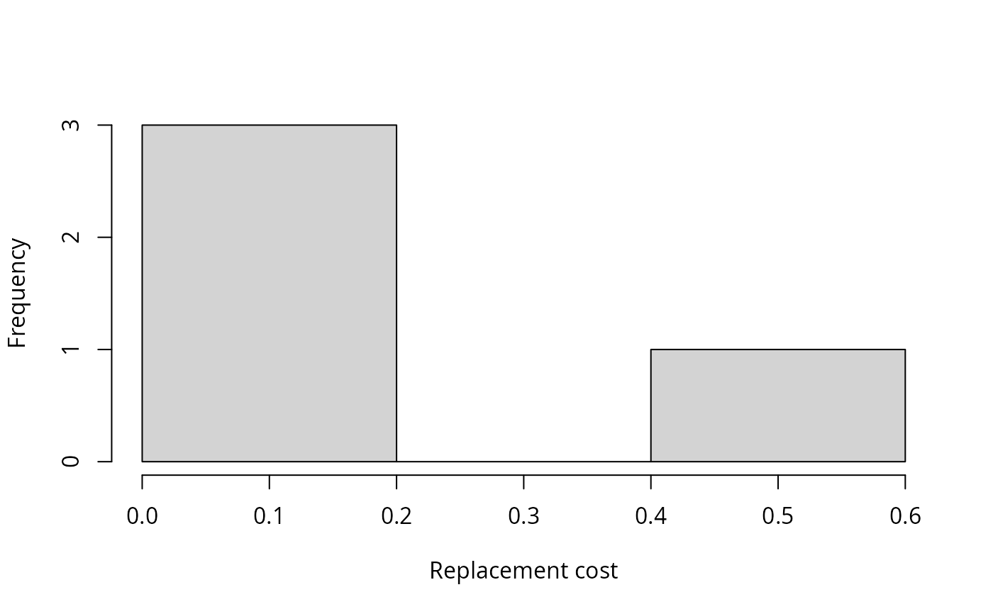
# plot histogram of replacement costs,
# with this objective, greater values indicate greater irreplaceability
hist(r$rep_cost, xlab = "Replacement cost", main = "")

# }
# }