Calculate the individual cost-effectiveness of each conservation project
in a project prioritization problem()
(Joseph, Maloney & Possingham 2009).
Arguments
- x
problem()object.
Value
A tibble::tibble() table containing the following
columns.
"project"charactername of each project"cost"numericcost of each project."benefit"numericbenefit for each project. For a given project, this is calculated as the difference between (i) the objective value for a solution containing all of the management actions associated with the project and all zero cost actions, and (ii) the objective value for a solution containing the baseline project."ce"numericcost-effectiveness of each project. For a given project, this is calculated as the difference between the the benefit for the project and the benefit for the baseline project, divided by the cost of the project. Note that the baseline project will have aNaNvalue because it has a zero cost."rank"numericrank for each project according to is cost-effectiveness value. The project with a rank of one is the most cost-effective project. Ties are accommodated using averages.
Details
Note that project cost-effectiveness cannot be calculated for problems with minimum set objectives because the objective function for these problems is to minimize cost and not maximize some measure of biodiversity persistence.
References
Joseph LN, Maloney RF & Possingham HP (2009) Optimal allocation of resources among threatened species: A project prioritization protocol. Conservation Biology, 23, 328–338.
See also
Other functions for evaluating solutions:
rank_importance(),
replacement_costs(),
solution_statistics()
Examples
# load data
data(sim_projects, sim_features, sim_actions)
# print project data
print(sim_projects)
#> # A tibble: 6 × 13
#> name success F1 F2 F3 F4 F5 F1_action F2_action
#> <chr> <dbl> <dbl> <dbl> <dbl> <dbl> <dbl> <lgl> <lgl>
#> 1 F1_project 0.919 0.791 NA NA NA NA TRUE FALSE
#> 2 F2_project 0.923 NA 0.888 NA NA NA FALSE TRUE
#> 3 F3_project 0.829 NA NA 0.502 NA NA FALSE FALSE
#> 4 F4_project 0.848 NA NA NA 0.690 NA FALSE FALSE
#> 5 F5_project 0.814 NA NA NA NA 0.617 FALSE FALSE
#> 6 baseline_proj… 1 0.298 0.250 0.0865 0.249 0.182 FALSE FALSE
#> # ℹ 4 more variables: F3_action <lgl>, F4_action <lgl>, F5_action <lgl>,
#> # baseline_action <lgl>
# print action data
print(sim_features)
#> # A tibble: 5 × 2
#> name weight
#> <chr> <dbl>
#> 1 F1 0.211
#> 2 F2 0.211
#> 3 F3 0.221
#> 4 F4 0.630
#> 5 F5 1.59
# print feature data
print(sim_actions)
#> # A tibble: 6 × 4
#> name cost locked_in locked_out
#> <chr> <dbl> <lgl> <lgl>
#> 1 F1_action 94.4 FALSE FALSE
#> 2 F2_action 101. FALSE FALSE
#> 3 F3_action 103. TRUE FALSE
#> 4 F4_action 99.2 FALSE FALSE
#> 5 F5_action 99.9 FALSE TRUE
#> 6 baseline_action 0 FALSE FALSE
# build problem
p <-
problem(
sim_projects, sim_actions, sim_features,
"name", "success", "name", "cost", "name"
) %>%
add_max_wtd_sum_objective(budget = 400) %>%
add_feature_weights("weight") %>%
add_binary_decisions()
# print problem
print(p)
#> Project Prioritization Problem
#> actions: F1_action, F2_action, F3_action, ... (6 actions)
#> projects: F1_project, F2_project, F3_project, ... (6 projects)
#> features: F1, F2, F3, ... (5 features)
#> action costs: continuous values (between 0 and 103.226)
#> project success: proportion values (between 0.814 and 1)
#> objective: maximum weighted sum objective
#> targets: none specified
#> weights: feature weights
#> constraints: none specified
#> decisions: binary decision
#> solver: none specified
# calculate cost-effectiveness of each project
pce <- project_cost_effectiveness(p)
# print project costs, benefits, and cost-effectiveness values
print(pce)
#> # A tibble: 6 × 6
#> project cost obj benefit ce rank
#> <chr> <dbl> <dbl> <dbl> <dbl> <dbl>
#> 1 F1_project 94.4 0.689 0.108 0.00114 4
#> 2 F2_project 101. 0.711 0.130 0.00129 3
#> 3 F3_project 103. 0.665 0.0841 0.000815 5
#> 4 F4_project 99.2 0.858 0.277 0.00279 2
#> 5 F5_project 99.9 1.23 0.653 0.00654 1
#> 6 baseline_project 0 0.581 0 NaN 6
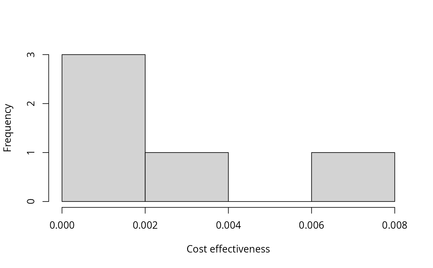
# plot histogram of cost-effectiveness values
hist(pce$ce, xlab = "Cost effectiveness", main = "")