Chapter 5 Spatial prioritizations

5.1 Introduction

Here we will develop prioritizations to identify priority areas for protected area establishment. Specifically, we will be using the prioritizr R package to generate prioritizations. Although other tools are also available for generating prioritizations – such as Marxan (Ardron et al. 2010), and Zonation (Moilanen et al. 2005) – it is beyond the scope of this workshop to examine them. Additionally, it is important to understand that software for generating prioritizations are decision support tools. This means that the software is designed to help you make decisions—it can’t make decisions for you.

5.2 Starting out simple

To start things off, let’s keep things simple. Let’s create a prioritization using the minimum set formulation of the reserve selection problem (Rodrigues et al. 2008). This formulation means that we want a solution that will meet the targets for our biodiversity features for minimum cost. Here, we will set 5% targets for each vegetation class and use the data in the cost column to specify acquisition costs. One advantage of prioritizr is that, unlike the Marxan decision support tool, we do not have calibrate (SPFs) to ensure the solution meets the targets. This is because – when using this formulation — prioritizr should always return solutions that meet the targets. Although we strongly recommend using Gurobi to solve problems (via add_gurobi_solver), we will use the HiGHS solver (via add_highs_solver) in this workshop since it is easier to install. This is because the Gurobi solver is much faster than the HiGHS solver (see here for installation instructions).

# print planning unit data
## note we use head() to show only show the first 6 rows
head(pu_data)

## Simple feature collection with 6 features and 5 fields
## Geometry type: MULTIPOLYGON
## Dimension:     XY
## Bounding box:  xmin: 303910.1 ymin: 5485840 xmax: 335610.4 ymax: 5502544
## Projected CRS: WGS 84 / UTM zone 55S
## # A tibble: 6 × 6
##      id  cost locked_in locked_out                                geom pa_status
##   <int> <dbl> <lgl>     <lgl>                       <MULTIPOLYGON [m]>     <dbl>
## 1     1  60.2 FALSE     TRUE       (((328497 5497704, 326783.8 550005…         0
## 2     2  19.9 FALSE     FALSE      (((307121.6 5490487, 305344.4 5492…         0
## 3     3  59.7 FALSE     TRUE       (((321726.1 5492382, 320111 549459…         0
## 4     4  32.4 FALSE     FALSE      (((304314.5 5494324, 304342.2 5494…         0
## 5     5  26.2 FALSE     FALSE      (((314958.5 5487057, 312336 549064…         0
## 6     6  51.3 FALSE     TRUE       (((327904.3 5491218, 326594.6 5493…         0

# create prioritization problem
p1 <-
  problem(pu_data, veg_data, cost_column = "cost") %>%
  add_min_set_objective() %>%
  add_relative_targets(0.05) %>% # 5% representation targets
  add_binary_decisions() %>%
  add_highs_solver(verbose = FALSE)

# print problem
print(p1)

## A conservation problem (<ConservationProblem>)
## ├•data
## │├•features:    "Banksia woodlands" , … (33 total)
## │└•planning units:
## │ ├•data:       <sftbl_dftbldata.frame> (1130 total)
## │ ├•costs:      continuous values (between 0.1925 and 61.9273)
## │ ├•extent:     298809.5764, 5167774.5993, 613818.7743, 5502543.7119 (xmin, ymin, xmax, ymax)
## │ └•CRS:        WGS 84 / UTM zone 55S (projected)
## ├•formulation
## │├•objective:   minimum set objective
## │├•penalties:   none specified
## │├•targets:     relative targets (between 0.05 and 0.05)
## │├•constraints: none specified
## │└•decisions:   binary decision
## └•optimization
##  ├•portfolio:   shuffle portfolio (`number_solutions` = 1, …)
##  └•solver:      highs solver (`gap` = 0.1, `time_limit` = 2147483647, …)
## # ℹ Use `summary(...)` to see complete formulation.

# solve problem
s1 <- solve(p1)

# print solution, the solution_1 column contains the solution values
# indicating if a planning unit is (1) selected or (0) not
## note we use head() to show only show the first 6 rows
head(s1)

## Simple feature collection with 6 features and 6 fields
## Geometry type: MULTIPOLYGON
## Dimension:     XY
## Bounding box:  xmin: 303910.1 ymin: 5485840 xmax: 335610.4 ymax: 5502544
## Projected CRS: WGS 84 / UTM zone 55S
## # A tibble: 6 × 7
##      id  cost locked_in locked_out pa_status solution_1
##   <int> <dbl> <lgl>     <lgl>          <dbl>      <dbl>
## 1     1  60.2 FALSE     TRUE               0          0
## 2     2  19.9 FALSE     FALSE              0          0
## 3     3  59.7 FALSE     TRUE               0          0
## 4     4  32.4 FALSE     FALSE              0          0
## 5     5  26.2 FALSE     FALSE              0          0
## 6     6  51.3 FALSE     TRUE               0          0
## # ℹ 1 more variable: geom <MULTIPOLYGON [m]>

# calculate number of planning units selected in the prioritization
sum(s1$solution_1)

## [1] 72

# calculate total cost of the prioritization
sum(s1$solution_1 * s1$cost)

## [1] 626.5873

# plot solution
plot(s1[, "solution_1"], pal = c("grey90", "darkgreen"))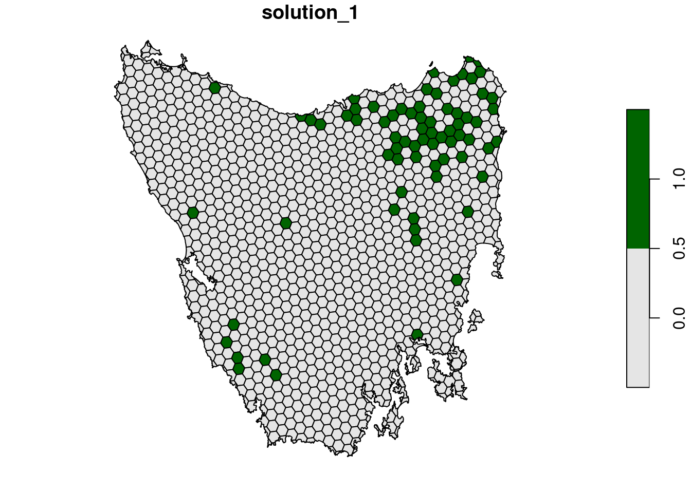

Now let’s examine the solution.

1. How many planing units were selected in the prioritization?
2. What proportion of planning units were selected in the prioritization?
3. Is there a pattern in the spatial distribution of the priority areas?
4. Can you verify that all of the targets were met in the prioritization (hint: feature_representation(p1, s1[, "solution_1"]))?

5.3 Adding complexity

Our first prioritization suffers many limitations, so let’s add additional constraints to the problem to make it more useful. First, let’s lock in planing units that are already by covered protected areas. If some vegetation communities are already secured inside existing protected areas, then we might not need to add as many new protected areas to the existing protected area system to meet their targets. Since our planning unit data (pu_data) already contains this information in the locked_in column, we can use this column name to specify which planning units should be locked in.

# create prioritization problem
p2 <-
  problem(pu_data, veg_data, cost_column = "cost") %>%
  add_min_set_objective() %>%
  add_relative_targets(0.05) %>%
  add_locked_in_constraints("locked_in") %>%
  add_binary_decisions() %>%
  add_highs_solver(verbose = FALSE)

# print problem
print(p2)

## A conservation problem (<ConservationProblem>)
## ├•data
## │├•features:    "Banksia woodlands" , … (33 total)
## │└•planning units:
## │ ├•data:       <sftbl_dftbldata.frame> (1130 total)
## │ ├•costs:      continuous values (between 0.1925 and 61.9273)
## │ ├•extent:     298809.5764, 5167774.5993, 613818.7743, 5502543.7119 (xmin, ymin, xmax, ymax)
## │ └•CRS:        WGS 84 / UTM zone 55S (projected)
## ├•formulation
## │├•objective:   minimum set objective
## │├•penalties:   none specified
## │├•targets:     relative targets (between 0.05 and 0.05)
## │├•constraints:
## ││└•1:          locked in constraints (257 planning units)
## │└•decisions:   binary decision
## └•optimization
##  ├•portfolio:   shuffle portfolio (`number_solutions` = 1, …)
##  └•solver:      highs solver (`gap` = 0.1, `time_limit` = 2147483647, …)
## # ℹ Use `summary(...)` to see complete formulation.

# solve problem
s2 <- solve(p2)

# plot solution
plot(s2[, "solution_1"], pal = c("grey90", "darkgreen"))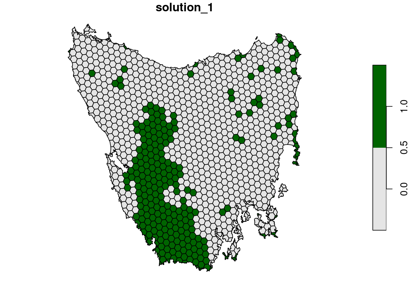

Let’s pretend that we talked to an expert on the vegetation communities in our study system and they recommended that a 30% target was needed for each vegetation class. So, equipped with this information, let’s set the targets to 20%.

# create prioritization problem
p3 <-
  problem(pu_data, veg_data, cost_column = "cost") %>%
  add_min_set_objective() %>%
  add_relative_targets(0.3) %>%
  add_locked_in_constraints("locked_in") %>%
  add_binary_decisions() %>%
  add_highs_solver(verbose = FALSE)

# print problem
print(p3)

## A conservation problem (<ConservationProblem>)
## ├•data
## │├•features:    "Banksia woodlands" , … (33 total)
## │└•planning units:
## │ ├•data:       <sftbl_dftbldata.frame> (1130 total)
## │ ├•costs:      continuous values (between 0.1925 and 61.9273)
## │ ├•extent:     298809.5764, 5167774.5993, 613818.7743, 5502543.7119 (xmin, ymin, xmax, ymax)
## │ └•CRS:        WGS 84 / UTM zone 55S (projected)
## ├•formulation
## │├•objective:   minimum set objective
## │├•penalties:   none specified
## │├•targets:     relative targets (between 0.3 and 0.3)
## │├•constraints:
## ││└•1:          locked in constraints (257 planning units)
## │└•decisions:   binary decision
## └•optimization
##  ├•portfolio:   shuffle portfolio (`number_solutions` = 1, …)
##  └•solver:      highs solver (`gap` = 0.1, `time_limit` = 2147483647, …)
## # ℹ Use `summary(...)` to see complete formulation.

# solve problem
s3 <- solve(p3)

# plot solution
plot(s3[, "solution_1"], pal = c("grey90", "darkgreen"))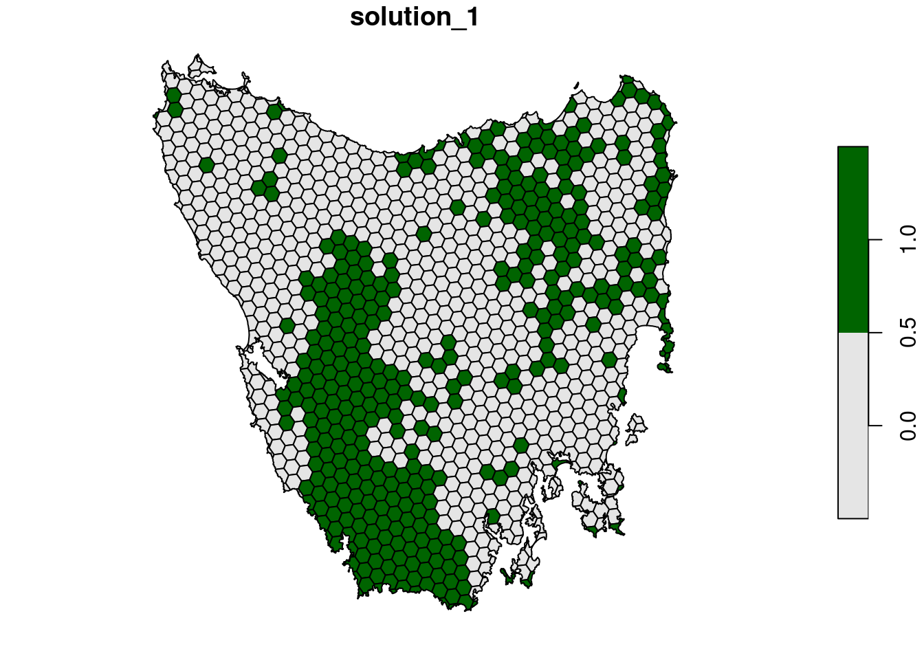

Next, let’s lock out highly degraded areas. Similar to before, this data is present in our planning unit data so we can use the locked_out column name to achieve this.

# create prioritization problem
p4 <-
  problem(pu_data, veg_data, cost_column = "cost") %>%
  add_min_set_objective() %>%
  add_relative_targets(0.3) %>%
  add_locked_in_constraints("locked_in") %>%
  add_locked_out_constraints("locked_out") %>%
  add_binary_decisions() %>%
  add_highs_solver(verbose = FALSE)

# print problem
print(p4)

## A conservation problem (<ConservationProblem>)
## ├•data
## │├•features:    "Banksia woodlands" , … (33 total)
## │└•planning units:
## │ ├•data:       <sftbl_dftbldata.frame> (1130 total)
## │ ├•costs:      continuous values (between 0.1925 and 61.9273)
## │ ├•extent:     298809.5764, 5167774.5993, 613818.7743, 5502543.7119 (xmin, ymin, xmax, ymax)
## │ └•CRS:        WGS 84 / UTM zone 55S (projected)
## ├•formulation
## │├•objective:   minimum set objective
## │├•penalties:   none specified
## │├•targets:     relative targets (between 0.3 and 0.3)
## │├•constraints:
## ││├•1:          locked in constraints (257 planning units)
## ││└•2:          locked out constraints (165 planning units)
## │└•decisions:   binary decision
## └•optimization
##  ├•portfolio:   shuffle portfolio (`number_solutions` = 1, …)
##  └•solver:      highs solver (`gap` = 0.1, `time_limit` = 2147483647, …)
## # ℹ Use `summary(...)` to see complete formulation.

# solve problem
s4 <- solve(p4)

# plot solution
plot(s4[, "solution_1"],  pal = c("grey90", "darkgreen"))

Now, let’s compare the solutions.

1. What is the cost of the planning units selected in s2, s3, and s4?
2. How many planning units are in s2, s3, and s4?
3. Do the solutions with more planning units have a greater cost? Why or why not?
4. Why does the first solution (s1) cost less than the second solution with protected areas locked into the solution (s2)?
5. Why does the third solution (s3) cost less than the fourth solution solution with highly degraded areas locked out (s4)?
6. Since planning units covered by existing protected areas have already been purchased, what is the cost for expanding the protected area system based on on the fourth prioritization (s4) (hint: total cost minus the cost of locked in planning units)?
7. What happens if you specify targets that exceed the total amount of vegetation in the study area and try to solve the problem? You can do this by modifying the code to make p4 with add_absolute_targets(1000) instead of add_relative_targets(0.3) and generating a new solution.

5.4 Penalizing fragmentation

Plans for protected area systems should facilitate gene flow and dispersal between individual reserves in the system (Beger et al. 2010; Hanson et al. 2022). However, the prioritizations we have made so far have been highly fragmented. Similar to the Marxan decision support tool, we can add penalties to our conservation planning problem to penalize fragmentation (i.e. total exposed boundary length) and we also need to set a useful penalty value when adding such penalties (akin to Marxan’s boundary length multiplier value; BLM) (Beyer et al. 2016). If we set our penalty value too low, then we will end up with a solution that is identical to the solution with no added penalties. If we set our penalty value too high, then prioritizr will take a long time to solve the problem and we will end up with a solution that contains lots of extra planning units that are not needed (since the penalty value is so high that minimizing fragmentation is more important than cost). As a rule of thumb, we generally want penalty values between 0.00001 and 0.01 but finding a useful penalty value requires calibration. The “correct” penalty value depends on the size of the planning units, the main objective values (e.g., cost values), and the effect of fragmentation on biodiversity persistence. Let’s create a new problem that is similar to our previous problem (p4) – except that it contains boundary length penalties and a slightly higher optimality gap to reduce runtime (default is 0.1) – and solve it. Since our planning unit data is in a spatial format (i.e., vector or raster data), prioritizr can automatically calculate the boundary data for us.

# create prioritization problem
p5 <-
  problem(pu_data, veg_data, cost_column = "cost") %>%
  add_min_set_objective() %>%
  add_boundary_penalties(penalty = 0.001) %>%
  add_relative_targets(0.3) %>%
  add_locked_in_constraints("locked_in") %>%
  add_locked_out_constraints("locked_out") %>%
  add_binary_decisions() %>%
  add_highs_solver(verbose = FALSE)

# print problem
print(p5)

## A conservation problem (<ConservationProblem>)
## ├•data
## │├•features:    "Banksia woodlands" , … (33 total)
## │└•planning units:
## │ ├•data:       <sftbl_dftbldata.frame> (1130 total)
## │ ├•costs:      continuous values (between 0.1925 and 61.9273)
## │ ├•extent:     298809.5764, 5167774.5993, 613818.7743, 5502543.7119 (xmin, ymin, xmax, ymax)
## │ └•CRS:        WGS 84 / UTM zone 55S (projected)
## ├•formulation
## │├•objective:   minimum set objective
## │├•penalties:
## ││└•1:          boundary penalties (`penalty` = 0.001, `edge_factor` = 0.5, …)
## │├•targets:     relative targets (between 0.3 and 0.3)
## │├•constraints:
## ││├•1:          locked in constraints (257 planning units)
## ││└•2:          locked out constraints (165 planning units)
## │└•decisions:   binary decision
## └•optimization
##  ├•portfolio:   shuffle portfolio (`number_solutions` = 1, …)
##  └•solver:      highs solver (`gap` = 0.1, `time_limit` = 2147483647, …)
## # ℹ Use `summary(...)` to see complete formulation.

# solve problem,
s5 <- solve(p5)

# print solution
## note we use head() to show only show the first 6 rows
head(s5)

## Simple feature collection with 6 features and 6 fields
## Geometry type: MULTIPOLYGON
## Dimension:     XY
## Bounding box:  xmin: 303910.1 ymin: 5485840 xmax: 335610.4 ymax: 5502544
## Projected CRS: WGS 84 / UTM zone 55S
## # A tibble: 6 × 7
##      id  cost locked_in locked_out pa_status solution_1
##   <int> <dbl> <lgl>     <lgl>          <dbl>      <dbl>
## 1     1  60.2 FALSE     TRUE               0          0
## 2     2  19.9 FALSE     FALSE              0          0
## 3     3  59.7 FALSE     TRUE               0          0
## 4     4  32.4 FALSE     FALSE              0          0
## 5     5  26.2 FALSE     FALSE              0          0
## 6     6  51.3 FALSE     TRUE               0          0
## # ℹ 1 more variable: geom <MULTIPOLYGON [m]>

# plot solution
plot(s5[, "solution_1"], pal = c("grey90", "darkgreen"))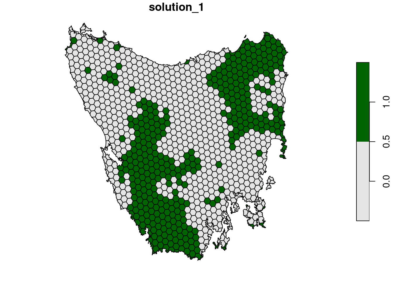

Now let’s compare the solutions to the problems with (s5) and without (s4) the boundary length penalties.

1. What is the cost the fourth (s4) and fifth (s5) solutions? Why does the fifth solution (s5) cost more than the fourth (s4) solution?
2. Try setting the penalty value to 0.000000001 (i.e. 1e-9) instead of 0.0005. What is the cost of the solution now? Is it different from the fourth solution (s4) (hint: try plotting the solutions to visualize them)? Is this is a useful penalty value? Why?
3. Try setting the penalty value to 0.5. What is the cost of the solution now? Is it different from the fourth solution (s4) (hint: try plotting the solutions to visualize them)? Is this a useful penalty value? Why?

5.5 Budget limited prioritizations

In the real-world, the funding available for conservation is often very limited. As a consequence, decision makers often need prioritizations where the total cost of priority areas does not exceed a budget. In our fourth prioritization (s4), we found that we would need to spend an additional $1334 million AUD to ensure that each vegetation community is adequately represented in the protected area system. But what if the funds available for establishing new protected areas were limited to $100 million AUD? In this case, we need a “budget limited prioritization”. Budget limited prioritizations aim to maximize some measure of conservation benefit subject to a budget (e.g., number of species with at least one occurrence in the protected area system, or phylogenetic diversity). Let’s create a prioritization that aims to minimize the target shortfalls as much as possible across all features whilst keeping within a pre-specified budget (following Jung et al. 2021).

# funds for additional land acquisition (same units as cost data)
funds <- 100

# calculate the total budget for the prioritization
budget <- funds + sum(s4$cost * s4$locked_in)
print(budget)

## [1] 8575.56

# create prioritization problem
p6 <-
  problem(pu_data, veg_data, cost_column = "cost") %>%
  add_min_shortfall_objective(budget) %>%
  add_relative_targets(0.3) %>%
  add_locked_in_constraints("locked_in") %>%
  add_locked_out_constraints("locked_out") %>%
  add_binary_decisions() %>%
  add_highs_solver(verbose = FALSE)

# print problem
print(p6)

## A conservation problem (<ConservationProblem>)
## ├•data
## │├•features:    "Banksia woodlands" , … (33 total)
## │└•planning units:
## │ ├•data:       <sftbl_dftbldata.frame> (1130 total)
## │ ├•costs:      continuous values (between 0.1925 and 61.9273)
## │ ├•extent:     298809.5764, 5167774.5993, 613818.7743, 5502543.7119 (xmin, ymin, xmax, ymax)
## │ └•CRS:        WGS 84 / UTM zone 55S (projected)
## ├•formulation
## │├•objective:   minimum shortfall objective (`budget` = 8575.5601)
## │├•penalties:   none specified
## │├•targets:     relative targets (between 0.3 and 0.3)
## │├•constraints:
## ││├•1:          locked in constraints (257 planning units)
## ││└•2:          locked out constraints (165 planning units)
## │└•decisions:   binary decision
## └•optimization
##  ├•portfolio:   shuffle portfolio (`number_solutions` = 1, …)
##  └•solver:      highs solver (`gap` = 0.1, `time_limit` = 2147483647, …)
## # ℹ Use `summary(...)` to see complete formulation.

# solve problem
s6 <- solve(p6)

# plot solution
plot(s6[, "solution_1"], pal = c("grey90", "darkgreen"))

# calculate feature representation
r6 <- eval_feature_representation_summary(p6, s6[, "solution_1"])

# calculate number of features with targets met
sum(r6$relative_held >= 0.3, na.rm = TRUE)

## [1] 15

# calculate average proportion of each feature represented by solution
mean(r6$relative_held, na.rm = TRUE)

## [1] 0.3238168

# find out which features have their targets met
print(r6$feature[r6$relative_held >= 0.3])

##  [1] "Boulders/rock with algae, lichen or scattered plants, or alpine fjaeldmarks"                           
##  [2] "Cool temperate rainforest"                                                                             
##  [3] "Eucalyptus open woodlands with shrubby understorey"                                                    
##  [4] "Eucalyptus tall open forests and open forests with ferns, herbs, sedges, rushes or wet tussock grasses"
##  [5] "Freshwater, dams, lakes, lagoons or aquatic plants"                                                    
##  [6] "Heathlands"                                                                                            
##  [7] "Leptospermum forests and woodlands"                                                                    
##  [8] "Low closed forest or tall closed shrublands (including Acacia, Melaleuca and Banksia)"                 
##  [9] "Mallee with a tussock grass understorey"                                                               
## [10] "Melaleuca shrublands and open shrublands"                                                              
## [11] "Mixed chenopod, samphire +/- forbs"                                                                    
## [12] "Other Acacia tall open shrublands and shrublands"                                                      
## [13] "Other open woodlands"                                                                                  
## [14] "Other shrublands"                                                                                      
## [15] "Sedgelands, rushs or reeds"

We can also add weights to specify that it is more important to meet the targets for certain features and less important for other features. A common approach for weighting features is to assign a greater importance to features with smaller spatial distributions. The rationale behind this weighting method is that features with smaller spatial distributions are at greater risk of extinction. So, let’s calculate some weights for our vegetation communities and see how weighting the features changes our prioritization.

# calculate weights as the log inverse number of grid cells that each vegetation
# class occupies, rescaled between 1 and 100
wts <- 1 / global(veg_data, "sum", na.rm = TRUE)[[1]]
wts <- scales::rescale(wts, to = c(1, 10))

# print the name of the feature with smallest weight
names(veg_data)[which.min(wts)]

## [1] "Eucalyptus open forests with a shrubby understorey"

# print the name of the feature with greatest weight
names(veg_data)[which.max(wts)]

## [1] "Mallee with a tussock grass understorey"

# plot histogram of weights
hist(wts, xlab = "Feature weights")

# create prioritization problem with weights
p7 <-
  problem(pu_data, veg_data, cost_column = "cost") %>%
  add_min_shortfall_objective(budget) %>%
  add_relative_targets(0.3) %>%
  add_feature_weights(wts) %>%
  add_locked_in_constraints("locked_in") %>%
  add_locked_out_constraints("locked_out") %>%
  add_binary_decisions() %>%
  add_highs_solver(verbose = FALSE)

# print problem
print(p7)

## A conservation problem (<ConservationProblem>)
## ├•data
## │├•features:    "Banksia woodlands" , … (33 total)
## │└•planning units:
## │ ├•data:       <sftbl_dftbldata.frame> (1130 total)
## │ ├•costs:      continuous values (between 0.1925 and 61.9273)
## │ ├•extent:     298809.5764, 5167774.5993, 613818.7743, 5502543.7119 (xmin, ymin, xmax, ymax)
## │ └•CRS:        WGS 84 / UTM zone 55S (projected)
## ├•formulation
## │├•objective:   minimum shortfall objective (`budget` = 8575.5601)
## │├•penalties:
## ││└•1:          feature weights (`weights` = asymmetric continuous values (non-zero values between 1 and 10))
## │├•targets:     relative targets (between 0.3 and 0.3)
## │├•constraints:
## ││├•1:          locked in constraints (257 planning units)
## ││└•2:          locked out constraints (165 planning units)
## │└•decisions:   binary decision
## └•optimization
##  ├•portfolio:   shuffle portfolio (`number_solutions` = 1, …)
##  └•solver:      highs solver (`gap` = 0.1, `time_limit` = 2147483647, …)
## # ℹ Use `summary(...)` to see complete formulation.

# solve problem
s7 <- solve(p7)

# plot solution
plot(s7[, "solution_1"], pal = c("grey90", "darkgreen"))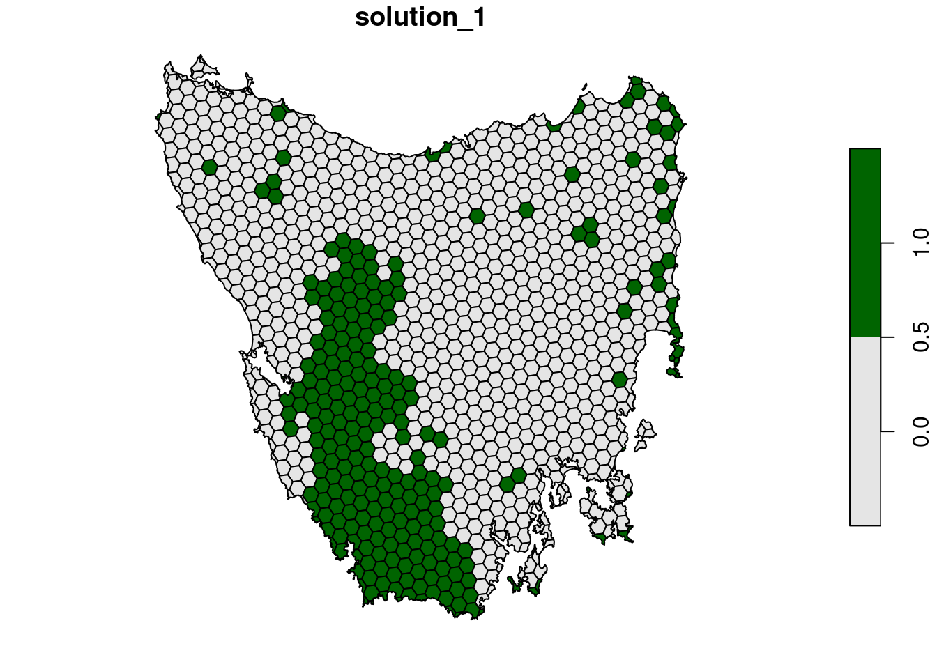

# calculate feature representation
r7 <- eval_feature_representation_summary(p7, s7[, "solution_1"])

# calculate number of features with targets met
sum(r7$relative_held >= 0.3, na.rm = TRUE)

## [1] 15

# calculate average proportion of each feature represented by solution
mean(r6$relative_held, na.rm = TRUE)

## [1] 0.3238168

# find out which features have their targets met when we add weights
print(r7$feature[r7$relative_held >= 0.3])

##  [1] "Banksia woodlands"                                                                    
##  [2] "Boulders/rock with algae, lichen or scattered plants, or alpine fjaeldmarks"          
##  [3] "Cool temperate rainforest"                                                            
##  [4] "Eucalyptus open woodlands with shrubby understorey"                                   
##  [5] "Freshwater, dams, lakes, lagoons or aquatic plants"                                   
##  [6] "Heathlands"                                                                           
##  [7] "Leptospermum forests and woodlands"                                                   
##  [8] "Low closed forest or tall closed shrublands (including Acacia, Melaleuca and Banksia)"
##  [9] "Mallee with a tussock grass understorey"                                              
## [10] "Melaleuca shrublands and open shrublands"                                             
## [11] "Mixed chenopod, samphire +/- forbs"                                                   
## [12] "Other Acacia tall open shrublands and shrublands"                                     
## [13] "Other open woodlands"                                                                 
## [14] "Other shrublands"                                                                     
## [15] "Sedgelands, rushs or reeds"

1. What is the name of the feature with the smallest weight?
2. What is the cost of the sixth (s6) and seventh (s7) solutions?
3. Does there seem to be a big difference in which planning units were selected in the sixth (s6) and seventh (s7) solutions?
4. Is there a difference between which features are adequately represented in the sixth (s6) and seventh (s7) solutions? If so, what is the difference?

References

Ardron, J.A., Possingham, H.P. & Klein, C.J. (2010). Marxan Good Practices Handbook , (2nd version)n. Pacific Marine Analysis; Research Association, Victoria, BC, Canada.

Beger, M., Linke, S., Watts, M., Game, E., Treml, E., Ball, I. & Possingham, H.P. (2010). Incorporating asymmetric connectivity into spatial decision making for conservation. Conservation Letters, 3, 359–368.

Beyer, H.L., Dujardin, Y., Watts, M.E. & Possingham, H.P. (2016). Solving conservation planning problems with integer linear programming. Ecological Modelling, 328, 14–22.

Hanson, J.O., Vincent, J., Schuster, R., Fahrig, L., Brennan, A., Martin, A.E., Hughes, J.S., Pither, R. & Bennett, J.R. (2022). A comparison of approaches for including connectivity in systematic conservation planning. Journal of Applied Ecology, 59, 2507–2519.

Jung, M., Arnell, A., Lamo, X. de, Garcı́a-Rangel, S., Lewis, M., Mark, J., Merow, C., Miles, L., Ondo, I., Pironon, S., Ravilious, C., Rivers, M., Schepaschenko, D., Tallowin, O., Soesbergen, A. van, Govaerts, R., Boyle, B.L., Enquist, B.J., Feng, X., Gallagher, R., Maitner, B., Meiri, S., Mulligan, M., Ofer, G., Roll, U., Hanson, J.O., Jetz, W., Marco, M.D., McGowan, J., Rinnan, D.S., Sachs, J.D., Lesiv, M., Adams, V.M., Andrew, S.C., Burger, J.R., Hannah, L., Marquet, P.A., McCarthy, J.K., Morueta-Holme, N., Newman, E.A., Park, D.S., Roehrdanz, P.R., Svenning, J.-C., Violle, C., Wieringa, J.J., Wynne, G., Fritz, S., Strassburg, B.B.N., Obersteiner, M., Kapos, V., Burgess, N., Schmidt-Traub, G. & Visconti, P. (2021). Areas of global importance for conserving terrestrial biodiversity, carbon and water. Nature Ecology and Evolution, 5, 1499–1509.

Moilanen, A., Franco, A.M.A., Early, R.I., Fox, R., Wintle, B. & Thomas, C.D. (2005). Prioritizing multiple-use landscapes for conservation: Methods for large multi-species planning problems. Proceedings of the Royal Society B: Biological Sciences, 272, 1885–1891.

Rodrigues, A.S., Cerdeira, J.O. & Gaston, K.J. (2008). Flexibility, efficiency, and accountability: Adapting reserve selection algorithms to more complex conservation problems. Ecography, 23, 565–574.