Plot a phylogram to visualize a project prioritization
Source:R/plot_solution_phylogram.R
plot_solution_phylogram.RdCreate a plot showing a phylogenetic tree (i.e., a "phylogram") to visualize
the probability that phylogenetic branches are expected to persist
into the future under a solution to a project prioritization problem().
Arguments
- x
problem()ormulti_problem()object.- solution
base::data.frame()ortibble::tibble()containing the solutions. Here, rows correspond to different solutions and columns correspond to different actions. Each column in the argument tosolutionshould be named according to a different action inx. Cell values indicate if an action is funded in a given solution or not, and should be either zero or one. Arguments tosolutioncan contain additional columns, though they will be ignored.- n
integersolution number to visualize. Since each row in the argument tosolutionscorresponds to a different solution, this argument should correspond to a row in the argument tosolutions. Defaults to 1.- symbol_hjust
numerichorizontal adjustment parameter to manually align the asterisks and dashes in the plot. Defaults to0.007. Increasing this parameter will shift the symbols further right. Please note that this parameter may require some tweaking to produce visually appealing publication quality plots.- return_data
logicalshould the underlying data used to create the plot be returned instead of the plot? Defaults toFALSE.
Value
A ggtree::ggtree() object, or a
tidytree::treedata() object if return_data is
TRUE.
Details
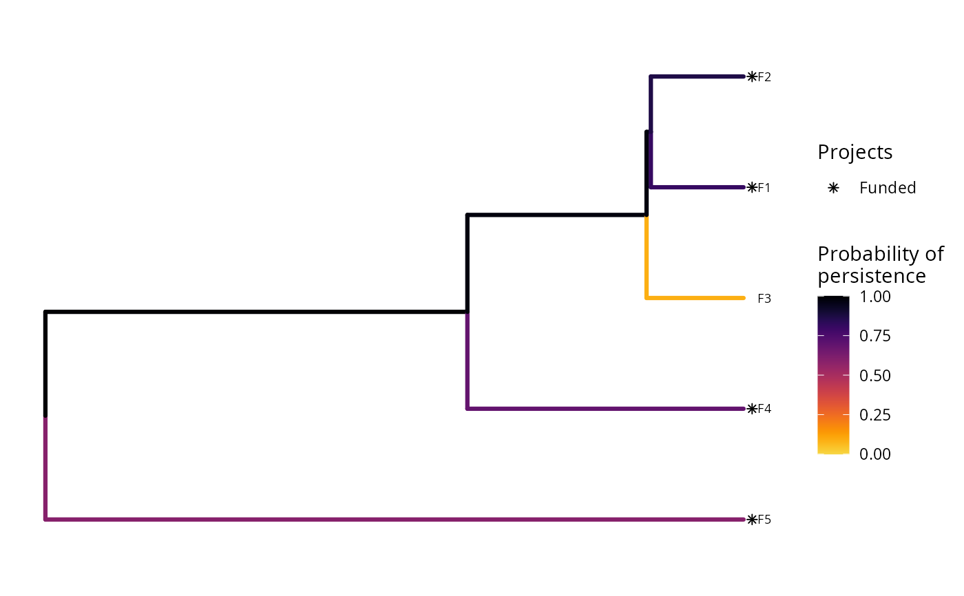
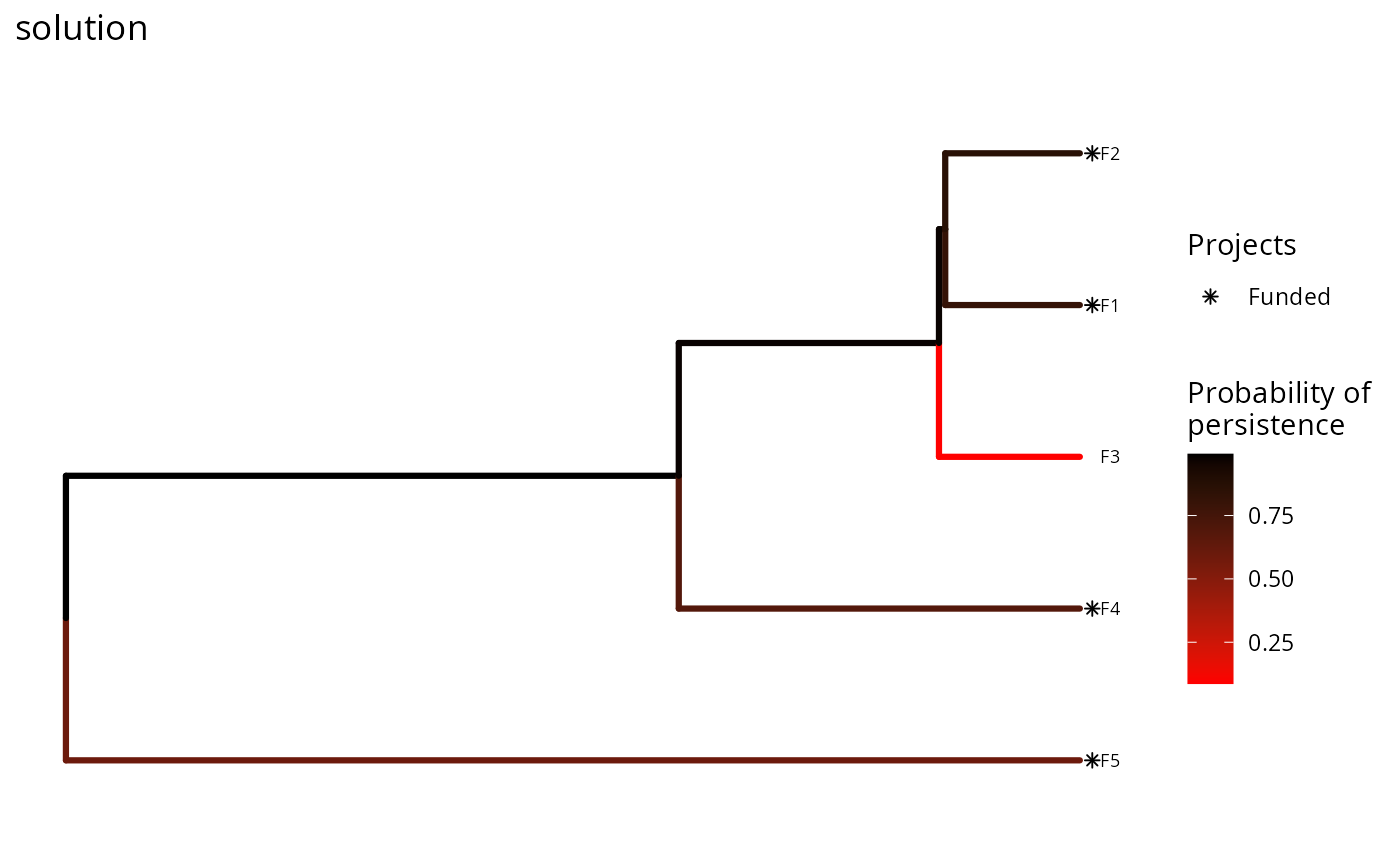
In this plot, each phylogenetic branch is colored according to probability that it is expected to persist into the future (per Faith 2008), based on the projects selected for funding by the solution. Features that directly benefit from at least a single completely funded project with a non-zero cost are depicted with an asterisk symbol. Additionally, features that indirectly benefit from funded projects – because they are associated with partially funded projects that have non-zero costs and share actions with at least one completely funded project – are depicted with an open circle symbol.
Dependencies
This function requires the ggtree (Yu et al. 2017). Since this package is distributed exclusively through Bioconductor, and is not available on the Comprehensive R Archive Network, please execute the following commands to install it:
If the installation process fails, please consult the package's online documentation.
References
Faith DP (2008) Threatened species and the potential loss of phylogenetic diversity: conservation scenarios based on estimated extinction probabilities and phylogenetic risk analysis. Conservation Biology, 22: 1461–1470.
Yu G, Smith DK, Zhu H, Guan Y, & Lam TTY (2017) ggtree: an R package for visualization and annotation of phylogenetic trees with their covariates and other associated data. Methods in Ecology and Evolution, 8: 28–36.
Examples
# set seed for reproducibility
set.seed(500)
# load the ggplot2 R package to customize plots
library(ggplot2)
data(sim_projects, sim_features, sim_actions)
# build problem
p <-
problem(
sim_projects, sim_actions, sim_features,
"name", "success", "name", "cost", "name"
) %>%
add_max_phylo_div_objective(budget = 400, sim_tree) %>%
add_binary_decisions() %>%
add_heuristic_solver(number_solutions = 10)
# solve problem
s <- solve(p)
# plot the first solution
plot(p, s)
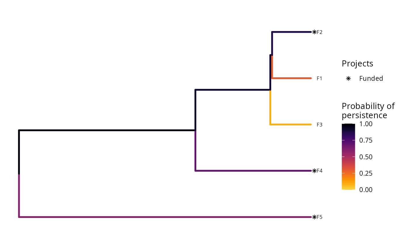
 # plot the second solution
plot(p, s, n = 2)
# plot the second solution
plot(p, s, n = 2)
 # since this function returns a ggplot2 plot object, we can customize the
# appearance of the plot using standard ggplot2 commands!
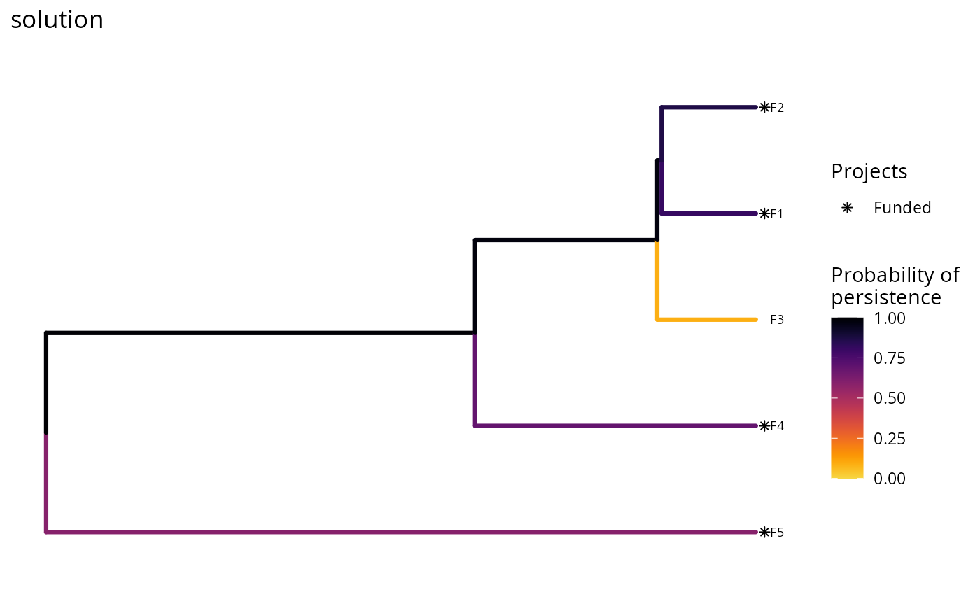
# for example, we can add a title
plot(p, s) + ggtitle("solution")
# since this function returns a ggplot2 plot object, we can customize the
# appearance of the plot using standard ggplot2 commands!
# for example, we can add a title
plot(p, s) + ggtitle("solution")
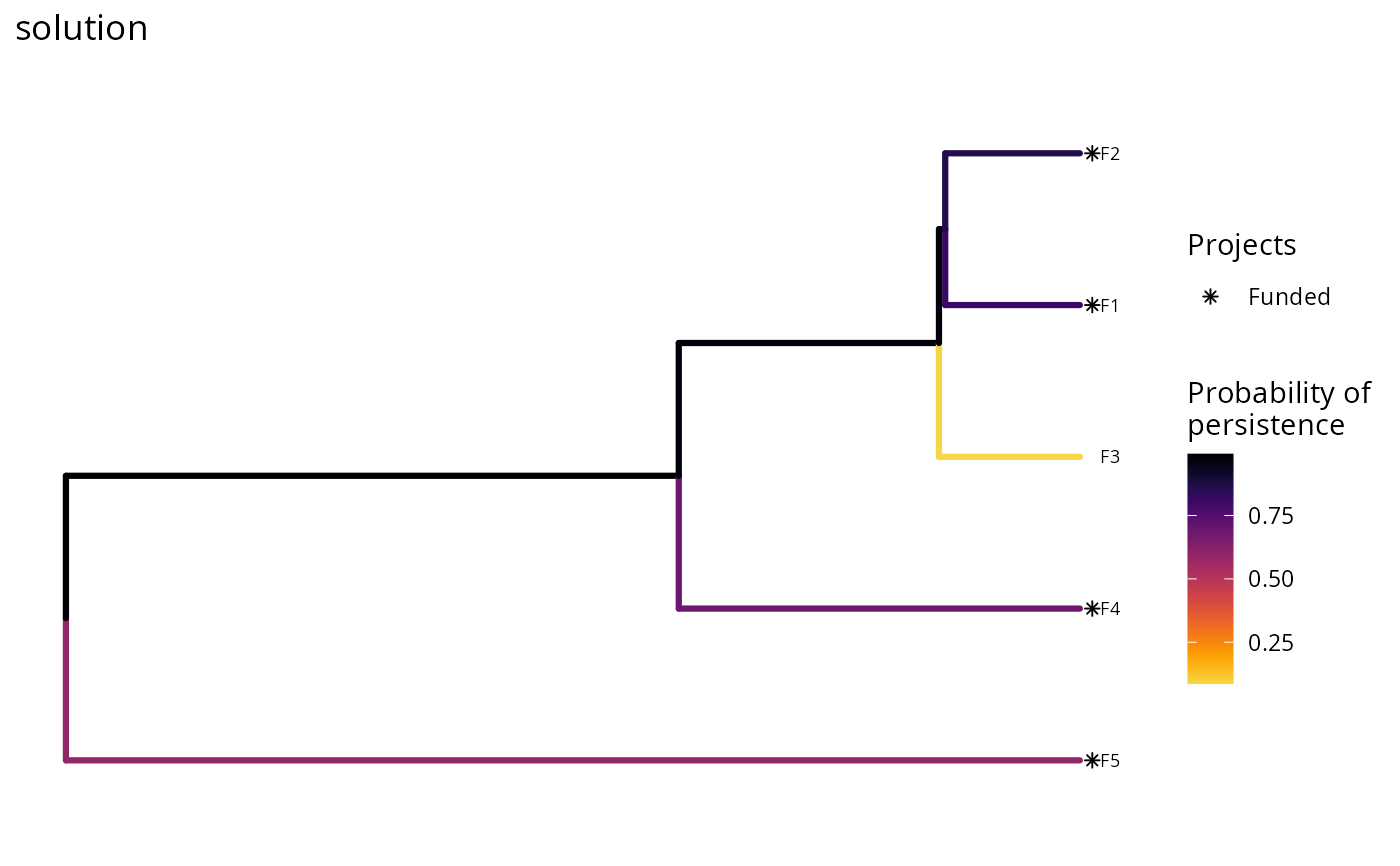
 # we could also also set the minimum and maximum values in the color ramp to
# correspond to those in the data, rather than being capped at 0 and 1
plot(p, s) +
scale_color_gradientn(
name = "Probability of\npersistence",
colors = viridisLite::inferno(150,
begin = 0,
end = 0.9,
direction = -1
)
) +
ggtitle("solution")
#> Scale for colour is already present.
#> Adding another scale for colour, which will replace the existing scale.
# we could also also set the minimum and maximum values in the color ramp to
# correspond to those in the data, rather than being capped at 0 and 1
plot(p, s) +
scale_color_gradientn(
name = "Probability of\npersistence",
colors = viridisLite::inferno(150,
begin = 0,
end = 0.9,
direction = -1
)
) +
ggtitle("solution")
#> Scale for colour is already present.
#> Adding another scale for colour, which will replace the existing scale.
 # we could also change the color ramp
plot(p, s) +
scale_color_gradient(
name = "Probability of\npersistence",
low = "red", high = "black"
) +
ggtitle("solution")
#> Scale for colour is already present.
#> Adding another scale for colour, which will replace the existing scale.
# we could also change the color ramp
plot(p, s) +
scale_color_gradient(
name = "Probability of\npersistence",
low = "red", high = "black"
) +
ggtitle("solution")
#> Scale for colour is already present.
#> Adding another scale for colour, which will replace the existing scale.
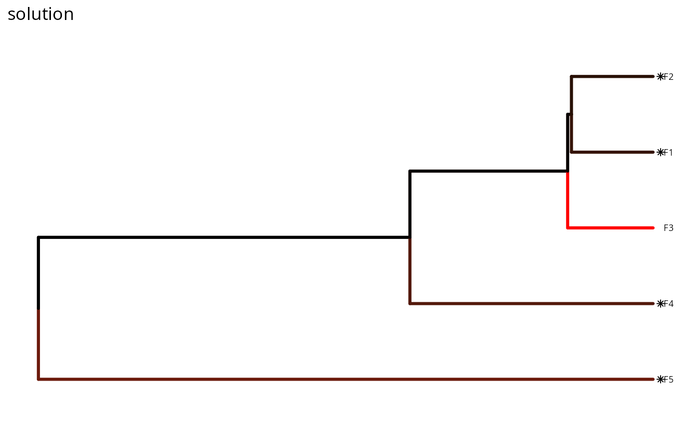
 # we could even hide the legend if desired
plot(p, s) +
scale_color_gradient(
name = "Probability of\npersistence",
low = "red", high = "black"
) +
theme(legend.position = "hide") +
ggtitle("solution")
#> Scale for colour is already present.
#> Adding another scale for colour, which will replace the existing scale.
# we could even hide the legend if desired
plot(p, s) +
scale_color_gradient(
name = "Probability of\npersistence",
low = "red", high = "black"
) +
theme(legend.position = "hide") +
ggtitle("solution")
#> Scale for colour is already present.
#> Adding another scale for colour, which will replace the existing scale.
 # we can also obtain the raw plotting data using return_data=TRUE
plot_data <- plot(p, s, return_data = TRUE)
print(plot_data)
#> 'treedata' S4 object'.
#>
#> ...@ phylo:
#>
#> Phylogenetic tree with 5 tips and 4 internal nodes.
#>
#> Tip labels:
#> F1, F2, F3, F4, F5
#> Node labels:
#> NA, NA, NA, NA
#>
#> Rooted; includes branch length(s).
#>
#> with the following features available:
#> 'status', 'prob'.
#>
#> # The associated data tibble abstraction: 9 × 5
#> # The 'node', 'label' and 'isTip' are from the phylo tree.
#> node label isTip status prob
#> <int> <chr> <lgl> <chr> <dbl>
#> 1 1 " F1" TRUE Funded 0.808
#> 2 2 " F2" TRUE Funded 0.865
#> 3 3 " F3" TRUE NA 0.0865
#> 4 4 " F4" TRUE Funded 0.688
#> 5 5 " F5" TRUE Funded 0.592
#> 6 6 " NA" FALSE NA NA
#> 7 7 " NA" FALSE NA 0.993
#> 8 8 " NA" FALSE NA 0.976
#> 9 9 " NA" FALSE NA 0.974
# we can also obtain the raw plotting data using return_data=TRUE
plot_data <- plot(p, s, return_data = TRUE)
print(plot_data)
#> 'treedata' S4 object'.
#>
#> ...@ phylo:
#>
#> Phylogenetic tree with 5 tips and 4 internal nodes.
#>
#> Tip labels:
#> F1, F2, F3, F4, F5
#> Node labels:
#> NA, NA, NA, NA
#>
#> Rooted; includes branch length(s).
#>
#> with the following features available:
#> 'status', 'prob'.
#>
#> # The associated data tibble abstraction: 9 × 5
#> # The 'node', 'label' and 'isTip' are from the phylo tree.
#> node label isTip status prob
#> <int> <chr> <lgl> <chr> <dbl>
#> 1 1 " F1" TRUE Funded 0.808
#> 2 2 " F2" TRUE Funded 0.865
#> 3 3 " F3" TRUE NA 0.0865
#> 4 4 " F4" TRUE Funded 0.688
#> 5 5 " F5" TRUE Funded 0.592
#> 6 6 " NA" FALSE NA NA
#> 7 7 " NA" FALSE NA 0.993
#> 8 8 " NA" FALSE NA 0.976
#> 9 9 " NA" FALSE NA 0.974