Add targets to a project prioritization that specify the desired expected outcome for each feature in the same units as the outcomes values. For example, if a feature has its outcome values expressed probabilities of persistence, then setting an absolute target of 0.1 means that the feature should ideally have a 10% chance of persistence.
Usage
add_absolute_targets(x, targets)

# S4 method for class 'ProjectProblem,numeric'
add_absolute_targets(x, targets)

# S4 method for class 'ProjectProblem,character'
add_absolute_targets(x, targets)Value
A problem() object with the targets added to it.
Details
Targets are used to specify a threshold minimum desirable expected outcome for each feature. These should ideally be set according to stakeholder requirements and expert knowledge. Please note that attempting to solve problems with objectives that require targets without specifying targets will throw an error.
The targets for a problem can be specified using the following options.
numericvalueThe value is used to set the target threshold for each feature. This option may be useful when all features should be assigned the same target threshold.
numericvectorEach value specifies a target threshold for each feature. The order of the values should correspond to the order of the features in
x.charactervalueThe value specifies the name of a column in the feature data (i.e., the argument to
featuresin theproblem()function). The target threshold for each feature is set according the column values.
See also
Other targets:
add_manual_targets(),
add_relative_targets()
Examples
# load data
data(sim_projects, sim_features, sim_actions)
# build problem with minimum set objective and targets that require each
# feature to have a 30% chance of persisting into the future
p1 <-
problem(
sim_projects, sim_actions, sim_features,
"name", "success", "name", "cost", "name"
) %>%
add_min_set_objective() %>%
add_absolute_targets(0.3) %>%
add_binary_decisions()
# print problem
print(p1)
#> Project Prioritization Problem
#> actions: F1_action, F2_action, F3_action, ... (6 actions)
#> projects: F1_project, F2_project, F3_project, ... (6 projects)
#> features: F1, F2, F3, ... (5 features)
#> action costs: continuous values (between 0 and 103.226)
#> project success: proportion values (between 0.814 and 1)
#> objective: minimum set objective
#> targets: absolute targets
#> weights: none specified
#> constraints: none specified
#> decisions: binary decision
#> solver: none specified
# build problem with minimum set objective and specify targets that require
# different levels of persistence for each feature
p2 <-
problem(
sim_projects, sim_actions, sim_features,
"name", "success", "name", "cost", "name"
) %>%
add_min_set_objective() %>%
add_absolute_targets(c(0.1, 0.2, 0.3, 0.4, 0.5)) %>%
add_binary_decisions()
# print problem
print(p2)
#> Project Prioritization Problem
#> actions: F1_action, F2_action, F3_action, ... (6 actions)
#> projects: F1_project, F2_project, F3_project, ... (6 projects)
#> features: F1, F2, F3, ... (5 features)
#> action costs: continuous values (between 0 and 103.226)
#> project success: proportion values (between 0.814 and 1)
#> objective: minimum set objective
#> targets: absolute targets
#> weights: none specified
#> constraints: none specified
#> decisions: binary decision
#> solver: none specified
# add a column name to the feature data with targets
sim_features$target <- c(0.1, 0.2, 0.3, 0.4, 0.5)
# build problem with minimum set objective and specify targets using
# column name in the feature data
p3 <-
problem(
sim_projects, sim_actions, sim_features,
"name", "success", "name", "cost", "name"
) %>%
add_min_set_objective() %>%
add_absolute_targets("target") %>%
add_binary_decisions()
# print problem
print(p3)
#> Project Prioritization Problem
#> actions: F1_action, F2_action, F3_action, ... (6 actions)
#> projects: F1_project, F2_project, F3_project, ... (6 projects)
#> features: F1, F2, F3, ... (5 features)
#> action costs: continuous values (between 0 and 103.226)
#> project success: proportion values (between 0.814 and 1)
#> objective: minimum set objective
#> targets: absolute targets
#> weights: none specified
#> constraints: none specified
#> decisions: binary decision
#> solver: none specified
# solve problems
s1 <- solve(p1)
#> Set parameter Username
#> Set parameter LicenseID to value 2806834
#> Set parameter TimeLimit to value 2147483647
#> Set parameter MIPGap to value 0
#> Set parameter ScaleFlag to value 2
#> Set parameter NumericFocus to value 1
#> Set parameter Presolve to value 2
#> Set parameter Threads to value 1
#> Set parameter PoolSolutions to value 1
#> Set parameter PoolSearchMode to value 2
#> Academic license - for non-commercial use only - expires 2027-04-14
#> Gurobi Optimizer version 13.0.1 build v13.0.1rc0 (linux64 - "Ubuntu 24.04.2 LTS")
#>
#> CPU model: 11th Gen Intel(R) Core(TM) i7-1185G7 @ 3.00GHz, instruction set [SSE2|AVX|AVX2|AVX512]
#> Thread count: 4 physical cores, 8 logical processors, using up to 1 threads
#>
#> Non-default parameters:
#> TimeLimit 2147483647
#> MIPGap 0
#> ScaleFlag 2
#> NumericFocus 1
#> Presolve 2
#> Threads 1
#> PoolSolutions 1
#> PoolSearchMode 2
#>
#> Optimize a model with 26 rows, 22 columns and 52 nonzeros (Min)
#> Model fingerprint: 0x21fb06c6
#> Model has 5 linear objective coefficients
#> Variable types: 0 continuous, 22 integer (22 binary)
#> Coefficient statistics:
#> Matrix range [9e-02, 1e+00]
#> Objective range [9e+01, 1e+02]
#> Bounds range [1e+00, 1e+00]
#> RHS range [3e-01, 1e+00]
#>
#> Found heuristic solution: objective 497.7671458
#> Presolve removed 25 rows and 20 columns
#> Presolve time: 0.00s
#> Presolved: 1 rows, 2 columns, 2 nonzeros
#> Variable types: 0 continuous, 2 integer (2 binary)
#>
#> Explored 0 nodes (0 simplex iterations) in 0.00 seconds (0.00 work units)
#> Thread count was 1 (of 8 available processors)
#>
#> Solution count 1: 497.767
#> No other solutions better than 497.767
#>
#> Optimal solution found (tolerance 0.00e+00)
#> Best objective 4.977671458279e+02, best bound 4.977671458279e+02, gap 0.0000%
s2 <- solve(p2)
#> Set parameter Username
#> Set parameter LicenseID to value 2806834
#> Set parameter TimeLimit to value 2147483647
#> Set parameter MIPGap to value 0
#> Set parameter ScaleFlag to value 2
#> Set parameter NumericFocus to value 1
#> Set parameter Presolve to value 2
#> Set parameter Threads to value 1
#> Set parameter PoolSolutions to value 1
#> Set parameter PoolSearchMode to value 2
#> Academic license - for non-commercial use only - expires 2027-04-14
#> Gurobi Optimizer version 13.0.1 build v13.0.1rc0 (linux64 - "Ubuntu 24.04.2 LTS")
#>
#> CPU model: 11th Gen Intel(R) Core(TM) i7-1185G7 @ 3.00GHz, instruction set [SSE2|AVX|AVX2|AVX512]
#> Thread count: 4 physical cores, 8 logical processors, using up to 1 threads
#>
#> Non-default parameters:
#> TimeLimit 2147483647
#> MIPGap 0
#> ScaleFlag 2
#> NumericFocus 1
#> Presolve 2
#> Threads 1
#> PoolSolutions 1
#> PoolSearchMode 2
#>
#> Optimize a model with 26 rows, 22 columns and 52 nonzeros (Min)
#> Model fingerprint: 0x09ccbe59
#> Model has 5 linear objective coefficients
#> Variable types: 0 continuous, 22 integer (22 binary)
#> Coefficient statistics:
#> Matrix range [9e-02, 1e+00]
#> Objective range [9e+01, 1e+02]
#> Bounds range [1e+00, 1e+00]
#> RHS range [1e-01, 1e+00]
#>
#> Found heuristic solution: objective 403.3678534
#> Presolve removed 19 rows and 14 columns
#> Presolve time: 0.00s
#> Presolved: 7 rows, 8 columns, 14 nonzeros
#> Variable types: 0 continuous, 8 integer (8 binary)
#> Root relaxation presolved: 2 rows, 3 columns, 4 nonzeros
#>
#>
#> Root relaxation: objective 3.023765e+02, 0 iterations, 0.00 seconds (0.00 work units)
#>
#> Nodes | Current Node | Objective Bounds | Work
#> Expl Unexpl | Obj Depth IntInf | Incumbent BestBd Gap | It/Node Time
#>
#> * 0 0 0 302.3764827 302.37648 0.00% - 0s
#>
#> Explored 1 nodes (0 simplex iterations) in 0.00 seconds (0.00 work units)
#> Thread count was 1 (of 8 available processors)
#>
#> Solution count 1: 302.376
#> No other solutions better than 302.376
#>
#> Optimal solution found (tolerance 0.00e+00)
#> Best objective 3.023764827378e+02, best bound 3.023764827378e+02, gap 0.0000%
s3 <- solve(p3)
#> Set parameter Username
#> Set parameter LicenseID to value 2806834
#> Set parameter TimeLimit to value 2147483647
#> Set parameter MIPGap to value 0
#> Set parameter ScaleFlag to value 2
#> Set parameter NumericFocus to value 1
#> Set parameter Presolve to value 2
#> Set parameter Threads to value 1
#> Set parameter PoolSolutions to value 1
#> Set parameter PoolSearchMode to value 2
#> Academic license - for non-commercial use only - expires 2027-04-14
#> Gurobi Optimizer version 13.0.1 build v13.0.1rc0 (linux64 - "Ubuntu 24.04.2 LTS")
#>
#> CPU model: 11th Gen Intel(R) Core(TM) i7-1185G7 @ 3.00GHz, instruction set [SSE2|AVX|AVX2|AVX512]
#> Thread count: 4 physical cores, 8 logical processors, using up to 1 threads
#>
#> Non-default parameters:
#> TimeLimit 2147483647
#> MIPGap 0
#> ScaleFlag 2
#> NumericFocus 1
#> Presolve 2
#> Threads 1
#> PoolSolutions 1
#> PoolSearchMode 2
#>
#> Optimize a model with 26 rows, 22 columns and 52 nonzeros (Min)
#> Model fingerprint: 0x09ccbe59
#> Model has 5 linear objective coefficients
#> Variable types: 0 continuous, 22 integer (22 binary)
#> Coefficient statistics:
#> Matrix range [9e-02, 1e+00]
#> Objective range [9e+01, 1e+02]
#> Bounds range [1e+00, 1e+00]
#> RHS range [1e-01, 1e+00]
#>
#> Found heuristic solution: objective 403.3678534
#> Presolve removed 19 rows and 14 columns
#> Presolve time: 0.00s
#> Presolved: 7 rows, 8 columns, 14 nonzeros
#> Variable types: 0 continuous, 8 integer (8 binary)
#> Root relaxation presolved: 2 rows, 3 columns, 4 nonzeros
#>
#>
#> Root relaxation: objective 3.023765e+02, 0 iterations, 0.00 seconds (0.00 work units)
#>
#> Nodes | Current Node | Objective Bounds | Work
#> Expl Unexpl | Obj Depth IntInf | Incumbent BestBd Gap | It/Node Time
#>
#> * 0 0 0 302.3764827 302.37648 0.00% - 0s
#>
#> Explored 1 nodes (0 simplex iterations) in 0.00 seconds (0.00 work units)
#> Thread count was 1 (of 8 available processors)
#>
#> Solution count 1: 302.376
#> No other solutions better than 302.376
#>
#> Optimal solution found (tolerance 0.00e+00)
#> Best objective 3.023764827378e+02, best bound 3.023764827378e+02, gap 0.0000%
# print solutions
print(s1)
#> # A tibble: 1 × 21
#> solution status cost obj F1_action F2_action F3_action F4_action F5_action
#> <int> <chr> <dbl> <dbl> <lgl> <lgl> <lgl> <lgl> <lgl>
#> 1 1 OPTIMAL 498. 498. TRUE TRUE TRUE TRUE TRUE
#> # ℹ 12 more variables: baseline_action <lgl>, F1_project <lgl>,
#> # F2_project <lgl>, F3_project <lgl>, F4_project <lgl>, F5_project <lgl>,
#> # baseline_project <lgl>, F1 <dbl>, F2 <dbl>, F3 <dbl>, F4 <dbl>, F5 <dbl>
print(s2)
#> # A tibble: 1 × 21
#> solution status cost obj F1_action F2_action F3_action F4_action F5_action
#> <int> <chr> <dbl> <dbl> <lgl> <lgl> <lgl> <lgl> <lgl>
#> 1 1 OPTIMAL 302. 302. FALSE FALSE TRUE TRUE TRUE
#> # ℹ 12 more variables: baseline_action <lgl>, F1_project <lgl>,
#> # F2_project <lgl>, F3_project <lgl>, F4_project <lgl>, F5_project <lgl>,
#> # baseline_project <lgl>, F1 <dbl>, F2 <dbl>, F3 <dbl>, F4 <dbl>, F5 <dbl>
print(s3)
#> # A tibble: 1 × 21
#> solution status cost obj F1_action F2_action F3_action F4_action F5_action
#> <int> <chr> <dbl> <dbl> <lgl> <lgl> <lgl> <lgl> <lgl>
#> 1 1 OPTIMAL 302. 302. FALSE FALSE TRUE TRUE TRUE
#> # ℹ 12 more variables: baseline_action <lgl>, F1_project <lgl>,
#> # F2_project <lgl>, F3_project <lgl>, F4_project <lgl>, F5_project <lgl>,
#> # baseline_project <lgl>, F1 <dbl>, F2 <dbl>, F3 <dbl>, F4 <dbl>, F5 <dbl>
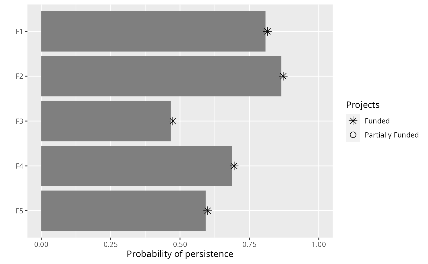
# plot solutions
plot(p1, s1)
 plot(p2, s2)
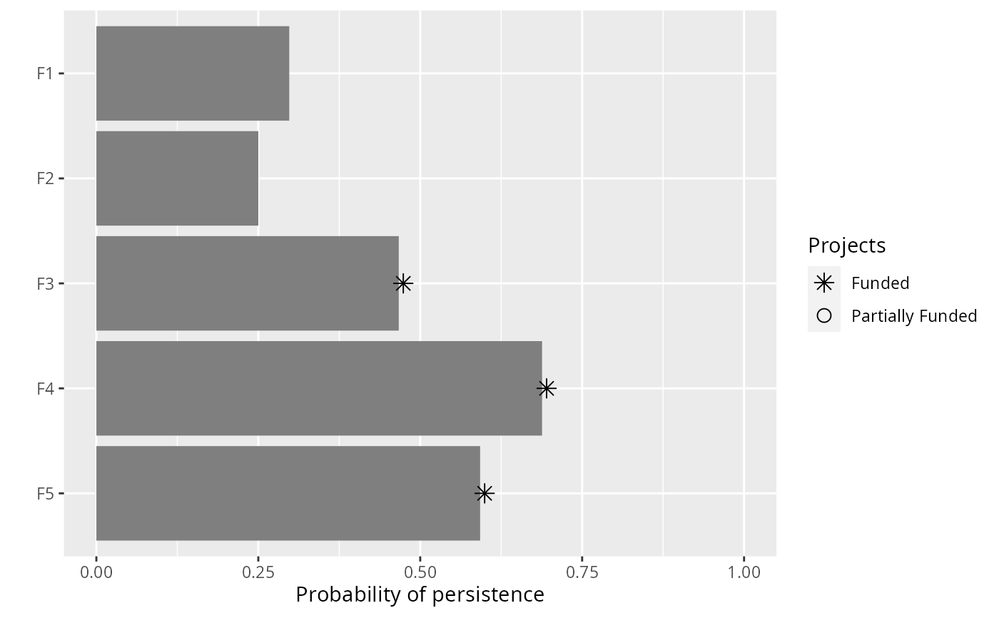 plot(p3, s3)
