Solve a conservation planning problem.
Arguments
- a
problem()object.- b
missing.
- ...
arguments passed to
compile().- run_checks
logicalflag indicating whether presolve checks should be run prior solving the problem. These checks are performed using thepresolve_check()function. Defaults toTRUE. Skipping these checks may reduce run time for large problems.- force
logicalflag indicating if an attempt to should be made to solve the problem even if potential issues were detected during the presolve checks. Defaults toFALSE.
Value
A numeric, matrix, data.frame, sf::st_sf(), or
terra::rast() object containing the solution to the problem.
Additionally, the returned object will have the following additional
attributes: "objective" containing the solution's objective,
"runtime" denoting the number of seconds that elapsed while solving
the problem, and "status" describing the status of the solution
(e.g., "OPTIMAL" indicates that the optimal solution was found).
Details
After formulating a conservation planning problem(),
it can be solved using an exact algorithm solver (see solvers
for available solvers). If no solver has been explicitly specified,
then the best available exact algorithm solver will be used by default
(see add_default_solver()). Although these exact algorithm
solvers will often display a lot of information that isn't really that
helpful (e.g., nodes, cutting planes), they do display information
about the progress they are making on solving the problem (e.g., the
performance of the best solution found at a given point in time). If
potential issues were detected during the
presolve checks (see presolve_check())
and the problem is being forcibly solved (i.e., with force = TRUE),
then it is also worth checking for any warnings displayed by the solver
to see if these potential issues are actually causing issues
(e.g., Gurobi can display warnings that include
"Warning: Model contains large matrix coefficient range" and
"Warning: Model contains large rhs").
Output format
This function will output solutions in a similar format to the
planning units associated with a. Specifically, it will return
solutions based on the following types of planning units.
ahasnumericplanning unitsThe solution will be returned as a
numericvector. Here, each element in the vector corresponds to a different planning unit. Note that if a portfolio is used to generate multiple solutions, then alistof suchnumericvectors will be returned.ahasmatrixplanning unitsThe solution will be returned as a
matrixobject. Here, rows correspond to different planning units, and columns correspond to different management zones. Note that if a portfolio is used to generate multiple solutions, then alistof suchmatrixobjects will be returned.ahasterra::rast()planning unitsThe solution will be returned as a
terra::rast()object. If the argument toxcontains multiple zones, then the object will have a different layer for each management zone. Note that if a portfolio is used to generate multiple solutions, then alistofterra::rast()objects will be returned.ahassf::sf(), ordata.frameplanning unitsThe solution will be returned in the same data format as the planning units. Here, each row corresponds to a different planning unit, and columns contain solutions. If the argument to
acontains a single zone, then the solution object will contain columns named by solution. Specifically, the column names containing the solution values be will named as"solution_XXX"where"XXX"corresponds to a solution identifier (e.g.,"solution_1"). If the argument toacontains multiple zones, then the columns containing solutions will be named as"solution_XXX_YYY"where"XXX"corresponds to the solution identifier and"YYY"is the name of the management zone (e.g.,"solution_1_zone1").
See also
See problem() to create conservation planning problems, and
presolve_check() to check problems for potential issues.
Also, see the category_layer() and category_vector() function to
reformat solutions that contain multiple zones.
Examples
# \dontrun{
# set seed for reproducibility
set.seed(500)
# load data
sim_pu_raster <- get_sim_pu_raster()
sim_pu_polygons <- get_sim_pu_polygons()
sim_features <- get_sim_features()
sim_zones_pu_raster <- get_sim_zones_pu_raster()
sim_zones_pu_polygons <- get_sim_zones_pu_polygons()
sim_zones_features <- get_sim_zones_features()
# build minimal conservation problem with raster data
p1 <-
problem(sim_pu_raster, sim_features) %>%
add_min_set_objective() %>%
add_relative_targets(0.1) %>%
add_binary_decisions() %>%
add_default_solver(verbose = FALSE)
# solve the problem
s1 <- solve(p1)
# print solution
print(s1)
#> class : SpatRaster
#> dimensions : 10, 10, 1 (nrow, ncol, nlyr)
#> resolution : 0.1, 0.1 (x, y)
#> extent : 0, 1, 0, 1 (xmin, xmax, ymin, ymax)
#> coord. ref. : Undefined Cartesian SRS
#> source(s) : memory
#> varname : sim_pu_raster
#> name : layer
#> min value : 0
#> max value : 1
# print attributes describing the optimization process and the solution
print(attr(s1, "objective"))
#> solution_1
#> 1987.399
print(attr(s1, "runtime"))
#> solution_1
#> 0.022
print(attr(s1, "status"))
#> solution_1
#> "OPTIMAL"
# calculate feature representation in the solution
r1 <- eval_feature_representation_summary(p1, s1)
print(r1)
#> # A tibble: 5 × 5
#> summary feature total_amount absolute_held relative_held
#> <chr> <chr> <dbl> <dbl> <dbl>
#> 1 overall feature_1 83.3 8.91 0.107
#> 2 overall feature_2 31.2 3.13 0.100
#> 3 overall feature_3 72.0 7.34 0.102
#> 4 overall feature_4 42.7 4.35 0.102
#> 5 overall feature_5 56.7 6.01 0.106
# plot solution
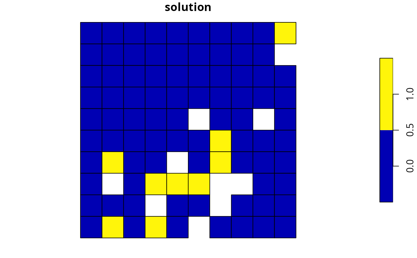
plot(s1, main = "solution", axes = FALSE)
 # build minimal conservation problem with polygon data
p2 <-
problem(sim_pu_polygons, sim_features, cost_column = "cost") %>%
add_min_set_objective() %>%
add_relative_targets(0.1) %>%
add_binary_decisions() %>%
add_default_solver(verbose = FALSE)
# solve the problem
s2 <- solve(p2)
# print solution
print(s2)
#> Simple feature collection with 90 features and 4 fields
#> Geometry type: POLYGON
#> Dimension: XY
#> Bounding box: xmin: 0 ymin: 0 xmax: 1 ymax: 1
#> Projected CRS: Undefined Cartesian SRS
#> # A tibble: 90 × 5
#> cost locked_in locked_out solution_1 geom
#> <dbl> <lgl> <lgl> <dbl> <POLYGON [m]>
#> 1 216. FALSE FALSE 0 ((0 1, 0.1 1, 0.1 0.9, 0 0.9, 0 1))
#> 2 213. FALSE FALSE 0 ((0.1 1, 0.2 1, 0.2 0.9, 0.1 0.9, 0.1 …
#> 3 207. FALSE FALSE 0 ((0.2 1, 0.3 1, 0.3 0.9, 0.2 0.9, 0.2 …
#> 4 209. FALSE TRUE 0 ((0.3 1, 0.4 1, 0.4 0.9, 0.3 0.9, 0.3 …
#> 5 214. FALSE FALSE 0 ((0.4 1, 0.5 1, 0.5 0.9, 0.4 0.9, 0.4 …
#> 6 214. FALSE FALSE 0 ((0.5 1, 0.6 1, 0.6 0.9, 0.5 0.9, 0.5 …
#> 7 210. FALSE FALSE 0 ((0.6 1, 0.7 1, 0.7 0.9, 0.6 0.9, 0.6 …
#> 8 211. FALSE TRUE 0 ((0.7 1, 0.8 1, 0.8 0.9, 0.7 0.9, 0.7 …
#> 9 210. FALSE FALSE 0 ((0.8 1, 0.9 1, 0.9 0.9, 0.8 0.9, 0.8 …
#> 10 204. FALSE FALSE 0 ((0.9 1, 1 1, 1 0.9, 0.9 0.9, 0.9 1))
#> # ℹ 80 more rows
# calculate feature representation in the solution
r2 <- eval_feature_representation_summary(p2, s2[, "solution_1"])
print(r2)
#> # A tibble: 5 × 5
#> summary feature total_amount absolute_held relative_held
#> <chr> <chr> <dbl> <dbl> <dbl>
#> 1 overall feature_1 74.5 8.05 0.108
#> 2 overall feature_2 28.1 2.83 0.101
#> 3 overall feature_3 64.9 6.65 0.103
#> 4 overall feature_4 38.2 3.87 0.101
#> 5 overall feature_5 50.7 5.41 0.107
# plot solution
plot(s2[, "solution_1"], main = "solution", axes = FALSE)
# build minimal conservation problem with polygon data
p2 <-
problem(sim_pu_polygons, sim_features, cost_column = "cost") %>%
add_min_set_objective() %>%
add_relative_targets(0.1) %>%
add_binary_decisions() %>%
add_default_solver(verbose = FALSE)
# solve the problem
s2 <- solve(p2)
# print solution
print(s2)
#> Simple feature collection with 90 features and 4 fields
#> Geometry type: POLYGON
#> Dimension: XY
#> Bounding box: xmin: 0 ymin: 0 xmax: 1 ymax: 1
#> Projected CRS: Undefined Cartesian SRS
#> # A tibble: 90 × 5
#> cost locked_in locked_out solution_1 geom
#> <dbl> <lgl> <lgl> <dbl> <POLYGON [m]>
#> 1 216. FALSE FALSE 0 ((0 1, 0.1 1, 0.1 0.9, 0 0.9, 0 1))
#> 2 213. FALSE FALSE 0 ((0.1 1, 0.2 1, 0.2 0.9, 0.1 0.9, 0.1 …
#> 3 207. FALSE FALSE 0 ((0.2 1, 0.3 1, 0.3 0.9, 0.2 0.9, 0.2 …
#> 4 209. FALSE TRUE 0 ((0.3 1, 0.4 1, 0.4 0.9, 0.3 0.9, 0.3 …
#> 5 214. FALSE FALSE 0 ((0.4 1, 0.5 1, 0.5 0.9, 0.4 0.9, 0.4 …
#> 6 214. FALSE FALSE 0 ((0.5 1, 0.6 1, 0.6 0.9, 0.5 0.9, 0.5 …
#> 7 210. FALSE FALSE 0 ((0.6 1, 0.7 1, 0.7 0.9, 0.6 0.9, 0.6 …
#> 8 211. FALSE TRUE 0 ((0.7 1, 0.8 1, 0.8 0.9, 0.7 0.9, 0.7 …
#> 9 210. FALSE FALSE 0 ((0.8 1, 0.9 1, 0.9 0.9, 0.8 0.9, 0.8 …
#> 10 204. FALSE FALSE 0 ((0.9 1, 1 1, 1 0.9, 0.9 0.9, 0.9 1))
#> # ℹ 80 more rows
# calculate feature representation in the solution
r2 <- eval_feature_representation_summary(p2, s2[, "solution_1"])
print(r2)
#> # A tibble: 5 × 5
#> summary feature total_amount absolute_held relative_held
#> <chr> <chr> <dbl> <dbl> <dbl>
#> 1 overall feature_1 74.5 8.05 0.108
#> 2 overall feature_2 28.1 2.83 0.101
#> 3 overall feature_3 64.9 6.65 0.103
#> 4 overall feature_4 38.2 3.87 0.101
#> 5 overall feature_5 50.7 5.41 0.107
# plot solution
plot(s2[, "solution_1"], main = "solution", axes = FALSE)
 # build multi-zone conservation problem with raster data
p3 <-
problem(sim_zones_pu_raster, sim_zones_features) %>%
add_min_set_objective() %>%
add_relative_targets(matrix(runif(15, 0.1, 0.2), nrow = 5, ncol = 3)) %>%
add_binary_decisions() %>%
add_default_solver(verbose = FALSE)
# solve the problem
s3 <- solve(p3)
# print solution
print(s3)
#> class : SpatRaster
#> dimensions : 10, 10, 3 (nrow, ncol, nlyr)
#> resolution : 0.1, 0.1 (x, y)
#> extent : 0, 1, 0, 1 (xmin, xmax, ymin, ymax)
#> coord. ref. : Undefined Cartesian SRS
#> source(s) : memory
#> varnames : sim_zones_pu_raster
#> sim_zones_pu_raster
#> sim_zones_pu_raster
#> names : zone_1, zone_2, zone_3
#> min values : 0, 0, 0
#> max values : 1, 1, 1
# calculate feature representation in the solution
r3 <- eval_feature_representation_summary(p3, s3)
print(r3)
#> # A tibble: 20 × 5
#> summary feature total_amount absolute_held relative_held
#> <chr> <chr> <dbl> <dbl> <dbl>
#> 1 overall feature_1 250. 47.1 0.188
#> 2 overall feature_2 93.6 17.9 0.191
#> 3 overall feature_3 216. 41.6 0.193
#> 4 overall feature_4 128. 23.7 0.185
#> 5 overall feature_5 170. 31.6 0.186
#> 6 zone_1 feature_1 83.3 16.5 0.198
#> 7 zone_1 feature_2 31.2 5.65 0.181
#> 8 zone_1 feature_3 72.0 14.2 0.198
#> 9 zone_1 feature_4 42.7 7.56 0.177
#> 10 zone_1 feature_5 56.7 11.1 0.197
#> 11 zone_2 feature_1 83.3 15.7 0.189
#> 12 zone_2 feature_2 31.2 6.03 0.193
#> 13 zone_2 feature_3 72.0 14.5 0.201
#> 14 zone_2 feature_4 42.7 7.82 0.183
#> 15 zone_2 feature_5 56.7 10.3 0.181
#> 16 zone_3 feature_1 83.3 14.8 0.178
#> 17 zone_3 feature_2 31.2 6.22 0.199
#> 18 zone_3 feature_3 72.0 13.0 0.180
#> 19 zone_3 feature_4 42.7 8.27 0.194
#> 20 zone_3 feature_5 56.7 10.2 0.180
# plot solution
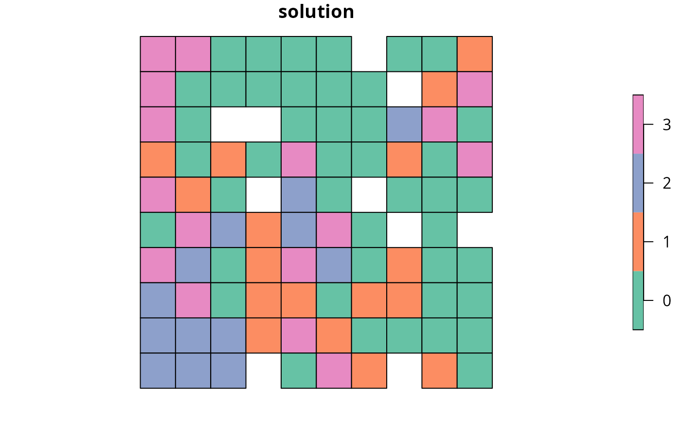
plot(category_layer(s3), main = "solution", axes = FALSE)
# build multi-zone conservation problem with raster data
p3 <-
problem(sim_zones_pu_raster, sim_zones_features) %>%
add_min_set_objective() %>%
add_relative_targets(matrix(runif(15, 0.1, 0.2), nrow = 5, ncol = 3)) %>%
add_binary_decisions() %>%
add_default_solver(verbose = FALSE)
# solve the problem
s3 <- solve(p3)
# print solution
print(s3)
#> class : SpatRaster
#> dimensions : 10, 10, 3 (nrow, ncol, nlyr)
#> resolution : 0.1, 0.1 (x, y)
#> extent : 0, 1, 0, 1 (xmin, xmax, ymin, ymax)
#> coord. ref. : Undefined Cartesian SRS
#> source(s) : memory
#> varnames : sim_zones_pu_raster
#> sim_zones_pu_raster
#> sim_zones_pu_raster
#> names : zone_1, zone_2, zone_3
#> min values : 0, 0, 0
#> max values : 1, 1, 1
# calculate feature representation in the solution
r3 <- eval_feature_representation_summary(p3, s3)
print(r3)
#> # A tibble: 20 × 5
#> summary feature total_amount absolute_held relative_held
#> <chr> <chr> <dbl> <dbl> <dbl>
#> 1 overall feature_1 250. 47.1 0.188
#> 2 overall feature_2 93.6 17.9 0.191
#> 3 overall feature_3 216. 41.6 0.193
#> 4 overall feature_4 128. 23.7 0.185
#> 5 overall feature_5 170. 31.6 0.186
#> 6 zone_1 feature_1 83.3 16.5 0.198
#> 7 zone_1 feature_2 31.2 5.65 0.181
#> 8 zone_1 feature_3 72.0 14.2 0.198
#> 9 zone_1 feature_4 42.7 7.56 0.177
#> 10 zone_1 feature_5 56.7 11.1 0.197
#> 11 zone_2 feature_1 83.3 15.7 0.189
#> 12 zone_2 feature_2 31.2 6.03 0.193
#> 13 zone_2 feature_3 72.0 14.5 0.201
#> 14 zone_2 feature_4 42.7 7.82 0.183
#> 15 zone_2 feature_5 56.7 10.3 0.181
#> 16 zone_3 feature_1 83.3 14.8 0.178
#> 17 zone_3 feature_2 31.2 6.22 0.199
#> 18 zone_3 feature_3 72.0 13.0 0.180
#> 19 zone_3 feature_4 42.7 8.27 0.194
#> 20 zone_3 feature_5 56.7 10.2 0.180
# plot solution
plot(category_layer(s3), main = "solution", axes = FALSE)
 # build multi-zone conservation problem with polygon data
p4 <-
problem(
sim_zones_pu_polygons, sim_zones_features,
cost_column = c("cost_1", "cost_2", "cost_3")
) %>%
add_min_set_objective() %>%
add_relative_targets(matrix(runif(15, 0.1, 0.2), nrow = 5, ncol = 3)) %>%
add_binary_decisions() %>%
add_default_solver(verbose = FALSE)
# solve the problem
s4 <- solve(p4)
# print solution
print(s4)
#> Simple feature collection with 90 features and 9 fields
#> Geometry type: POLYGON
#> Dimension: XY
#> Bounding box: xmin: 0 ymin: 0 xmax: 1 ymax: 1
#> Projected CRS: Undefined Cartesian SRS
#> # A tibble: 90 × 10
#> cost_1 cost_2 cost_3 locked_1 locked_2 locked_3 solution_1_zone_1
#> <dbl> <dbl> <dbl> <lgl> <lgl> <lgl> <dbl>
#> 1 216. 183. 205. FALSE FALSE FALSE 0
#> 2 213. 189. 210. FALSE FALSE FALSE 0
#> 3 207. 194. 215. TRUE FALSE FALSE 0
#> 4 209. 198. 219. FALSE FALSE FALSE 0
#> 5 214. 200. 221. FALSE FALSE FALSE 0
#> 6 214. 203. 225. FALSE FALSE FALSE 0
#> 7 211. 209. 223. FALSE FALSE FALSE 0
#> 8 210. 212. 222. TRUE FALSE FALSE 1
#> 9 204. 218. 214. FALSE FALSE FALSE 1
#> 10 213. 183. 206. FALSE FALSE FALSE 0
#> # ℹ 80 more rows
#> # ℹ 3 more variables: solution_1_zone_2 <dbl>, solution_1_zone_3 <dbl>,
#> # geom <POLYGON [m]>
# calculate feature representation in the solution
r4 <- eval_feature_representation_summary(
p4, s4[, c("solution_1_zone_1", "solution_1_zone_2", "solution_1_zone_3")]
)
print(r4)
#> # A tibble: 20 × 5
#> summary feature total_amount absolute_held relative_held
#> <chr> <chr> <dbl> <dbl> <dbl>
#> 1 overall feature_1 225. 37.5 0.166
#> 2 overall feature_2 83.9 14.6 0.174
#> 3 overall feature_3 195. 34.0 0.174
#> 4 overall feature_4 114. 18.4 0.161
#> 5 overall feature_5 154. 25.1 0.163
#> 6 zone_1 feature_1 75.1 12.8 0.170
#> 7 zone_1 feature_2 28.0 4.63 0.165
#> 8 zone_1 feature_3 65.0 10.6 0.163
#> 9 zone_1 feature_4 38.0 6.29 0.165
#> 10 zone_1 feature_5 51.2 8.88 0.174
#> 11 zone_2 feature_1 75.1 11.0 0.146
#> 12 zone_2 feature_2 28.0 5.26 0.188
#> 13 zone_2 feature_3 65.0 10.7 0.165
#> 14 zone_2 feature_4 38.0 6.49 0.171
#> 15 zone_2 feature_5 51.2 7.27 0.142
#> 16 zone_3 feature_1 75.1 13.7 0.182
#> 17 zone_3 feature_2 28.0 4.75 0.170
#> 18 zone_3 feature_3 65.0 12.7 0.195
#> 19 zone_3 feature_4 38.0 5.62 0.148
#> 20 zone_3 feature_5 51.2 8.93 0.175
# create new column representing the zone id that each planning unit
# was allocated to in the solution
s4$solution <- category_vector(
s4[, c("solution_1_zone_1", "solution_1_zone_2", "solution_1_zone_3")]
)
s4$solution <- factor(s4$solution)
# plot solution
plot(s4[, "solution"])
# build multi-zone conservation problem with polygon data
p4 <-
problem(
sim_zones_pu_polygons, sim_zones_features,
cost_column = c("cost_1", "cost_2", "cost_3")
) %>%
add_min_set_objective() %>%
add_relative_targets(matrix(runif(15, 0.1, 0.2), nrow = 5, ncol = 3)) %>%
add_binary_decisions() %>%
add_default_solver(verbose = FALSE)
# solve the problem
s4 <- solve(p4)
# print solution
print(s4)
#> Simple feature collection with 90 features and 9 fields
#> Geometry type: POLYGON
#> Dimension: XY
#> Bounding box: xmin: 0 ymin: 0 xmax: 1 ymax: 1
#> Projected CRS: Undefined Cartesian SRS
#> # A tibble: 90 × 10
#> cost_1 cost_2 cost_3 locked_1 locked_2 locked_3 solution_1_zone_1
#> <dbl> <dbl> <dbl> <lgl> <lgl> <lgl> <dbl>
#> 1 216. 183. 205. FALSE FALSE FALSE 0
#> 2 213. 189. 210. FALSE FALSE FALSE 0
#> 3 207. 194. 215. TRUE FALSE FALSE 0
#> 4 209. 198. 219. FALSE FALSE FALSE 0
#> 5 214. 200. 221. FALSE FALSE FALSE 0
#> 6 214. 203. 225. FALSE FALSE FALSE 0
#> 7 211. 209. 223. FALSE FALSE FALSE 0
#> 8 210. 212. 222. TRUE FALSE FALSE 1
#> 9 204. 218. 214. FALSE FALSE FALSE 1
#> 10 213. 183. 206. FALSE FALSE FALSE 0
#> # ℹ 80 more rows
#> # ℹ 3 more variables: solution_1_zone_2 <dbl>, solution_1_zone_3 <dbl>,
#> # geom <POLYGON [m]>
# calculate feature representation in the solution
r4 <- eval_feature_representation_summary(
p4, s4[, c("solution_1_zone_1", "solution_1_zone_2", "solution_1_zone_3")]
)
print(r4)
#> # A tibble: 20 × 5
#> summary feature total_amount absolute_held relative_held
#> <chr> <chr> <dbl> <dbl> <dbl>
#> 1 overall feature_1 225. 37.5 0.166
#> 2 overall feature_2 83.9 14.6 0.174
#> 3 overall feature_3 195. 34.0 0.174
#> 4 overall feature_4 114. 18.4 0.161
#> 5 overall feature_5 154. 25.1 0.163
#> 6 zone_1 feature_1 75.1 12.8 0.170
#> 7 zone_1 feature_2 28.0 4.63 0.165
#> 8 zone_1 feature_3 65.0 10.6 0.163
#> 9 zone_1 feature_4 38.0 6.29 0.165
#> 10 zone_1 feature_5 51.2 8.88 0.174
#> 11 zone_2 feature_1 75.1 11.0 0.146
#> 12 zone_2 feature_2 28.0 5.26 0.188
#> 13 zone_2 feature_3 65.0 10.7 0.165
#> 14 zone_2 feature_4 38.0 6.49 0.171
#> 15 zone_2 feature_5 51.2 7.27 0.142
#> 16 zone_3 feature_1 75.1 13.7 0.182
#> 17 zone_3 feature_2 28.0 4.75 0.170
#> 18 zone_3 feature_3 65.0 12.7 0.195
#> 19 zone_3 feature_4 38.0 5.62 0.148
#> 20 zone_3 feature_5 51.2 8.93 0.175
# create new column representing the zone id that each planning unit
# was allocated to in the solution
s4$solution <- category_vector(
s4[, c("solution_1_zone_1", "solution_1_zone_2", "solution_1_zone_3")]
)
s4$solution <- factor(s4$solution)
# plot solution
plot(s4[, "solution"])
 # }
# }